5. COLUMN DENSITIES, LINE BROADENING, AND KINEMATICS
There are basically two major issues to be explored regarding the nature of Mg II absorbing clouds. The first is the question of their internal motions, and their chemical and ionization conditions. How both these conditions are related to their spatial location with respect to the stellar material in galaxies is a higher order issue that must wait to be addressed when a large database of galaxy properties and high resolution spectra of high ionization transitions become available. The second major issue is the question of the cloud kinematics. Whether the cloud motions are systematic or random has implications for the lifetimes of the clouds, which in turn forces an explanation of either the sustenance of individual clouds or of a reservoir of clouds in absorbing systems. Otherwise, it is difficult to understand the apparent lack of evolution in the cross section of Mg II absorbers over a several Gyr period.
For given chemical and ionization conditions, certain relationships between Mg II, Fe II, and Mg I column densities are expected. The Doppler b parameter, obtained by the VP decompositions, can be used to infer the cloud temperatures and the level of possible non-thermal internal motions. The clustering kinematics of the clouds can be studied by investigating the cloud-cloud clustering and how the column densities and other inferred cloud properties depend upon the velocity of a cloud. It is important to remember that the study of the gas kinematics is entirely on a relative footing (between clouds in systems), since there is no absolute velocity scale. There are two pieces of information about the stellar content of the galaxies that is critical to a deeper appreciation of the connections between absorbing gas kinematics and galaxy kinematics. The first is a very accurate systemic redshift of the galaxies ( < 30 km/s is desired). These redshift provide the velocity zero point for the kinematics. The second is a measure of the stellar dynamics, either via rotation curves (Vogt et al. 1996) for spirals or doublet splitting for ellipticals (Koo et al. 1995).
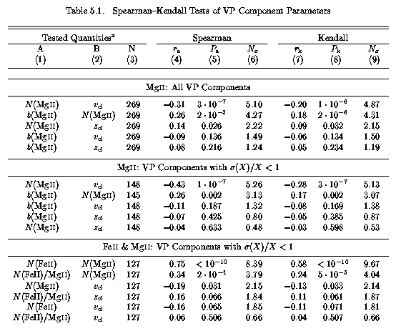
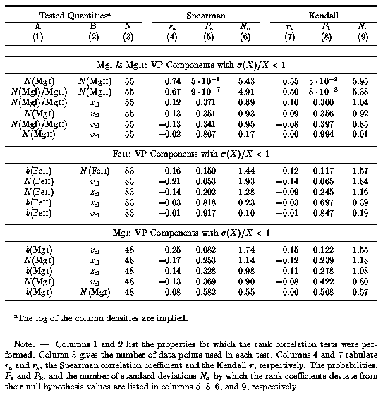
Given that relationships between VP parameters hold the promise of revealing somewhat detailed information from which inferences can be drawn, it follows that trends between these parameters should be sought. Spearman-Kendall tests were performed on the various VP parameters in order to search for correlations. The results of these tests are presented in Table 5.1. Six groups of tests are tabulated. The first two are identical except that, for the second of the two, only those components that had less than unity fractional errors in both their column densities and Doppler b parameters were included. In the cases where the VP parameters of two different ions were tested, the included data are those for which less than unity fractional errors were found for both ions. The results are ordered in decreasing significance level for each group of tests.
Table 5.1
5.1 THE Mg II, Fe II, and Mg I COLUMN DENSITIES
In Figure 5.1, the Fe II and Mg I VP column densities are plotted verses the Mg II column densities. Only components for which the fractional errors are less than unity in both ions are plotted. Both N(Fe II) and N(Mg I) are strongly correlated with N(Mg II). The Spearman-Kendall tests yield a ~9-sigma and a ~6-sigma result, respectively, with vanishing probabilities that correlations of with these significance levels could happen by chance (see Table 5.1).
Figure 5.1
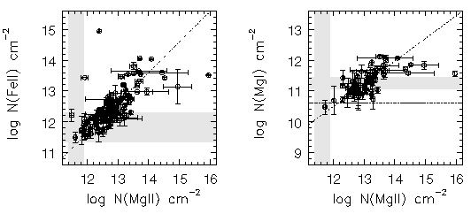
FIG. 5.1 --- (left panel) The Fe II VP verses Mg II VP column densities. --- (right panel) The Mg I VP verses Mg II VP column densities. The selected components have have fractional errors less than unity. The shaded regions give the range from total completeness in the highest S/N spectrum to the lowest S/N spectrum in Sample B for unblended lines. The dash-dot lines are the maximum likelihood fits and the dotted line at log N(MgI) = 10.5 cm^-2 is the 20% completeness contour of the lowest S/N spectrum.
Assuming a linear relationship in log - log, the best fit parameters were determined using a chi^2 minimization that allowed for errors in both the "y" and "x" data, and using a maximum likelihood method, called a local M estimator (minimizes the absolute deviations between the fit and the data) (Press et al. 1992). The best fit parameters are

using chi^2 minimization, and

using the maximum likelihood method. For the Fe II fit, chi^2 = 33, and for the Mg I fit the mean absolute deviation is 0.27. The Mg I chi^2 fit yielded chi^2 = 23, but the fit was heavily influenced by the single point at log N(Mg II) ~ 16 cm^-2, and resulted in an unacceptable slope for the bulk of the data. The large chi^2 values are indicative of a level of scatter that is real, rather than being an artifact of the measurement uncertainties. The linear fits to the Fe II - Mg II VP column densities obtained with the Blending Simulations yielded chi^2 ~ 10 independent of the signal to noise in the spectra (see Figure 4.14). It was then suggested that a chi^2 larger than this value would be suggestive of intrinsic scatter in the data. If follows that the N(Fe II) and N(Mg I) to N(Mg II) ratios vary either from system to system, or within systems, since the data include the many components within systems.
Exactly where the locus of column densities lie in the log(X) - log(Mg II) plane depends on a number of factors, including but not limited to the metallicity of the gas, the relative abundance of the elements in the gaseous phase (either due to depletion effects or to local chemical evolution histories), and the ionization conditions. It is unfortunate that Fe II and Mg I relative to Mg II are both less than ideal indicators. Iron can suffer significant levels of depletion (as can Mg) and has an ionization potential that is not that different than Mg II (roughly 1 eV higher). Mg I, on the other hand, undergoes a charge exchange reaction with H II that remains uncertain in its overall effect on the equilibrium balance of Mg I. Even so, in absence of direct knowledge of the H I column densities in the absorbing clouds, photoionization modeling can be used to at least attempt to constrain the overall chemical and ionization conditions of the gas.
Following the approach detailed in Steidel (1990), a grid of CLOUDY (Ferland 1980) photoionization models were constructed. Several authors have applied photoionization models to QSO absorption line systems (Bergeron & Stansinska 1986; Chaffee 1986; Morris 1986}; Bechtold, Green, & York 1987; Petitjean, Bergeron, & Puget 1992; Bergeron et al. 1994; Giroux, Sutherland, & Shull 1994; Dittman & Koppen 1995; Viegas & Friaca 1995; Giroux & Shull 1997). Dittmann & Koppen developed an algorithm to determine the optimal ionization parameters from the existing, yet large, database of low resolution observations. Since all these authors were working with low resolution data, they were actually finding the, ionization conditions within the dominant ionizing component in each system. With the VP decomposition of the HIRES data, there is now the opportunity to study ionization conditions in more detail.
Assuming that the clouds are photoionized, and are not collisionally ionized, a main question to be addressed is whether the clouds are radiated by stellar continuum from the local galaxy or if they are are radiated by the UV meta-galactic background flux. The shape of the ionizing continuum plays a central role in the resulting ionization conditions within Mg II absorbing clouds and it remains uncertain. The secondary question is whether any of the observed column densities are consistent with collisional ionization. For this work, only a somewhat limited study is presented.
Following Bergeron & Stasinska (1986), Dittmann & Koppen (1995), and Steidel (1990), the clouds are modeled as constant density plane parallel slabs, illuminated on one side by the ionizing radiation field. Each cloud was modeled using the ionization parameter

where n_gamma is the number density of photons with energy greater than 1 Rydberg incident on the cloud and n_H is the number density of hydrogen atoms in the gas. Varying U is equivalent to varying either n_H for constant n_gamma, or varying n_gamma for constant n_H. What needs to be specified, however, is the shape of the ionizing spectrum. In order to bracket the extreme cases of local stellar radiation and of the meta-galactic UV background, two slopes are examined and the results compared to the observed column densities. The UV background is approximated with a power law of slope alpha = - 1.5 (Bergeron & Stasinska 1986; Bechtold et al. 1987; Bergeron et al. 1994). This ionizing field is relatively hard. The stellar ionizing field is assumed to be a simple blackbody with T = 30,000 K. Such a field is taken to represent typical B stars, though UV line blanketing in the photospheres of these stars renders the stellar spectra even softer than the thermal field.
Each cloud is defined by its H I column density, metallicity, and ionization parameter. The metallicity has been set to 0.01 solar. The output of CLOUDY is the observed column densities of the various stages of ionization for the elements under study. For all clouds, the observed column densities are proportional to the metallicity. If the cloud is optically thin to hydrogen ionizing photons, then the shape of the spectrum is unchanged inside the clouds and the clouds have no spatial ionization structure. For this case, the homology relation

holds. Thus, for a given model cloud, the resulting observed column density scales with the H I column density and metallicity (one cannot discern the effects of changing either quantity).
In Figure 5.2 and Figure 5.3 the quantities log N(Mg I) - log N(Mg II) (upper panel) and log N(Fe II) - log N(Mg II) (lower panel) verses log N(Mg II) are plotted. Both Figures also show a grid of CLOUDY models for the predicted locus of the plotted data as a function of log U and log N(H I) in steps of 0.5 dex. Figure 5.2 illustrates the grid for the UV meta-galactic flux and Figure 5.3 illustrates the grid for the T = 30,000 K thermal ionizing flux. In addition, the quantities log N(Mg I) - log N(Mg II) verses log N(Fe II) - log N(Mg II) are plotted in Figure 5.4. Both CLOUDY grids are illustrated as solid curves. The predicted locus of column density ratios are also given for a collisional ionization model as a function of the gas temperature. The collisional ionization model points were taken from Tytler et al. (1987) and are the locus of points expected if absorption arises in H II regions.
Based upon the log N(Fe II) - log N(Mg II) data, it appears that the power law ionizing continuum is consistent with the data for log U < -3.0 with the bulk of the clouds having 17.0 < log N(H I) < 18.0 cm^-2. The trend for clouds with implied log N(H I) < 17.0 cm^-2 to be clustered with smaller log U is consistent with expectations. If the clouds are ionized by a thermal radiation source, then the implied hydrogen neutral column density is log N(H I) < 17.0 cm^-2 for log U < -1.0. This would imply that log N(Mg II) = 13.0 cm^-2 clouds arise in optically thin hydrogen clouds, which is difficult to understand in view of the fact that Mg II systems with these column densities are almost always associated with Lyman limit systems (Bechtold et al. 1984; Lanzetta 1988).
Figure 5.2
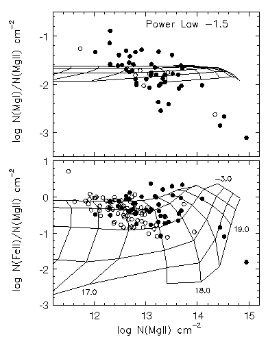
FIG. 5.2 --- The quantities $\log N(\hbox{\MgI})/\log N(\hbox{\MgII})$ and $\log N(\hbox{\FeII})/\log N(\hbox{\MgII})$ verses $\log N(\hbox{\MgII})$. The CLOUDY grids are for an assumed power law $-1.5$ ionization field. The vertical curves are lines of constant $\log N(\hbox{\HI})$ in steps of 0.5, starting with $\log N(\hbox{\HI}) = 20$~{\cm2} at the right most curve. The horizontal curves are lines of constant ionization parameter, $\log U$, which decreases from $-1.5$ in steps of 0.5 going upward.
However, the power law model places tight constraints on the allowed values of log N(Mg I) - log N(Mg II) as a function of N(Mg II). As can be seen in Figure 5.2, roughly half of the VP component column densities are scattered outside the model predictions. Note that the model grid shows virtually no dependence on Mg II column density. However, the observed log N(Mg I) - log N(Mg II) is strongly correlated with log N(Mg II). The Spearman-Kendall tests yield a ~5-sigma result with a probability of P~ 10^-8 that this significance level could happen by chance (see Table 5.1). However, careful examination of the VP fits from which the column densities were derived revealed that the data with log N(Mg I) - log N(Mg II) < -2.5 were always the central components in broad and saturated Mg II profiles. It is likely that these particular data points suffer from an overestimation of the Mg II column density, which pushes each data point downward and to the right in the diagram. If points with log N(Mg II) > 14 cm^-2 are removed from the sample, a strong correlation of log N(Mg I) - log N(Mg II) with log N(Mg II) is still present, in that the Spearman-Kendall tests yield 4-sigma result with P = (6 x 10^-5 , 3 x 10^-5}) that no correlation is consistent with the data. On the other hand, the data with log N(Mg II) < 12.4 cm^-2 may suffer from the fact that the Doppler parameter is not as well constrained for small N(Mg I). Following examination of the VP components that occupy the upper left of the diagram, it is concluded that these data points are robust for the most part. Thus, the anti-correlation between log N(Mg I) - log N(Mg II) with log N(Mg II) is accepted as real.
For the thermal model, it is reasonable to obtain log N(Mg I) - log N(Mg II) < -2.5, but, as with the power law model, it is still not possible to obtain log N(Mg I) - log N(Mg II) > -1.6. Many of the data points that occupy this region of Figure 5.2 and Figure 5.3 are secure VP fits, though there 1-sigma uncertainties do not render them inconsistent with the photoionization grids (the error in the vertical direction can be estimated by examining Figure 5.1 and introducing a factor of sqrt(2). The VP components with log N(Mg I) - log N(Mg II) > -1.6 may be indicate that the charge transfer reaction between H II and Mg I has a smaller importance relative to photoionization processes than have been applied in photoionization models (e.g. Petitjean & Bergeron 1990; Bergeron & Stasinska 1986).
Figure 5.3
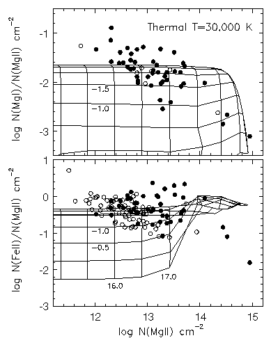
FIG. 5.3 --- The quantities $\log N(\hbox{\MgI})/\log N(\hbox{\MgII})$ and $\log N(\hbox{\FeII})/\log N(\hbox{\MgII})$ verses $\log N(\hbox{\MgII})$. The CLOUDY grids are for a $T=30,000$~K thermal ionization field. The vertical curves are lines of constant $\log N(\hbox{\HI})$ in steps of 0.5, starting with $\log N(\hbox{\HI}) = 20$~{\cm2} at the right most curve. The horizontal curves are lines of constant ionization parameter, $\log U$, which decreases in steps of 0.5 going upward.
A direct comparison of the two extreme photoionization models with a collisional excitation model is presented in Figure 5.4. As mentioned above, those data points that are consistent with the thermal model likely have their N(Mg II) overestimated. If the N(Mg II) were smaller, the data points would tend to move upward parallel to the lines of constant log N(H I) on the thermal model grid. Again, the data that are somewhat difficult to explain are those with log N(Mg I) - log N(Mg II) > -1.6, given that they lie equally distant from the power-law photoionization grid and the locus expected for collisionally excited clouds.
Figure 5.4
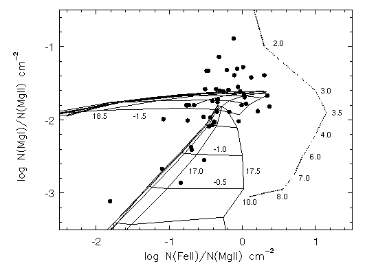
FIG. 5.4 --- The quantities $\log N(\hbox{\MgI})/\log N(\hbox{\MgII})$ and $\log N(\hbox{\FeII})/\log N(\hbox{\MgII})$ verses $\log N(\hbox{\MgII})$. The CLOUDY grids are for a $T=30,000$~K thermal ionization field. The vertical curves are lines of constant $\log N(\hbox{\HI})$ in steps of 0.5, starting with $\log N(\hbox{\HI}) = 20$~{\cm2} at the right most curve. The horizontal curves are lines of constant ionization parameter, $\log U$, which decreases in steps of 0.5 going upward.
5.1.1 Distribution of VP Component Column Densities
Petitjean & Bergeron (1990) used a power law probability distribution to describe the number density of Mg II systems per unit column density and obtained a maximum likelihood slope of f(N) ~ N^(-1.0 +/- 0.1) in the range 12.0 < log N(Mg II) < 14.3 cm^-2. The resolution of their data was ~30 km/s, and it is likely that their best fit slope is affected by unresolved VP components. The expected trend is that the number of large column density components would decrease, being redistributed into a larger number of smaller column density components. Thus, the measured slope obtained with higher resolution data is likely steeper.
[This Section Abridged]. For the HIRES data, the maximum likelihood method was used to obtain the slope and normalization of the power-law probability distribution,

where m, the total number of "clouds" from the VP decomposition, normalizes f(N) over the observed data.
In reality, there is no a priori upper limit to the observed column densities, so that it could be argued that the normalization should extend to infinity since this is the "observed" range in practice. The value of the normalization constant would then be systematically underestimated, since the total number density of clouds out to infinite column is not known. Thus, the normalization constant, C, and its uncertainty, are computed over the range of the observed data. For the purpose of further assessing uncertainty in the deduced value of delta, both normalizations were performed.
Figure 5.5
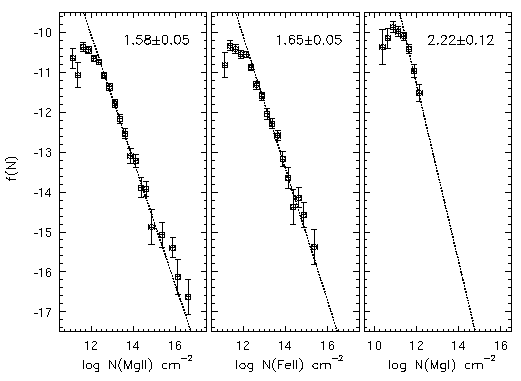
FIG. 5.5 --- The distribution function, $f(N) \propto N ^{-\delta}$, for the {\MgII} (left panel), the {\FeII} (central panel), and the {\MgI} (right panel) VP column densities. The dotted lines are the maximum likelihood fits to the unbinned data.
In Figure 5.5, the maximum likelihood power law distribution functions are shown for Mg II, Fe II, and Mg I. A lower column density was applied in each case, based upon the values suggested by the Blending Simulations Section 4.5. The cutoffs were varied to see if the value of \delta converged to a single value as the cutoff was increased (as was done for the simulations; see Table 4.1. The final Mg II was found to be 0.2 dex higher than that found for the Blending Simulations. This may be due to the fact that the effects of blending are more severe in the real data than in the simulations. It is likely that such an effect would result if the velocity clustering of the VP components is tighter in the real data than in the simulated data. The Fe II and Mg I cutoffs were found to be roughly equal to the completeness cutoffs for unblended features. This suggest that the completeness of detected Fe II and Mg I absorption features do not suffer significantly from blending. The final cutoffs were log N(Mg II) = 12.5 cm^-2, log N(Fe II) = 12.3 cm^-2, and log N(Mg I) = 11.5 cm^-2. The maximum likelihood values were

for Mg II,

for Fe II, and

for Mg I.
To guide the choice of the "best" maximum likelihood fit, a Kolmogorov-Smirnov (KS) test (Press et al. 1992) to the normalized cumulative distribution function was performed for trial values of the cutoff column density. The normalized cumulative distribution of column densities, which ranges from zero at N = N_min to unity at N = N_max, is given by

which can be expressed as

When the KS statistic,

where P( < N ) is the functional form of the measured cumulative distribution function, is minimized for a given cutoff column density, it is suggestive of a "best" choice of N_min. For the Mg II column density distribution with the log N(Mg II) = 12.5 cm^-2 cutoff, the KS statistic was D = 0.06 with a probability P_KS = 0.73 that a value this small would occur by chance. A value of P_KS < 0.01 for a given D would be suggestive that the P( < N ) is not consistent with n( < N ). For the Mg I column density distribution with the log N(Mg I) = 11.5 cm^-2 cutoff, the KS statistic was D = 0.14 with a probability P_KS = 0.49 that a value this small would occur by chance. A total of 147 data points and 31 data points were included in these tests for Mg II and Mg I, respectively. For both these distributions, the results provided good indicators for the choice of N_min, and thus the resulting value of delta.
The Fe II distribution, on the other hand, was not as clear cut. The simulations have shown that the completeness limit for unblended Fe II lines is log N(Fe II) = 12.3 cm^-2 for the signal to noise ratios in the HIRES spectra. Blending of components increases this value by ~0.3 dex. The KS statistic for the cutoff log N = 12.3 cm^-2 and the maximum likelihood value of delta = 1.65 is D = 0.16 with P_KS = 0.02. Increasing the cutoff, which yields larger delta, yields larger D and smaller P_KS (the results are less consistent with the data). However, if the cutoff log N = 12.3 cm^-2 is used and the value "assigned" to delta is 1.58 (that found for the Mg II), the KS statistic is D = 0.10 with P_KS = 0.15. The upshot is that the value of delta for the Fe II column may be more consistent with delta = 1.58. The implication is that the Fe II distribution may in fact be consistent with the Mg II distribution.
However, it is clear that the distribution of Mg I column densities has a significantly steeper power. As concluded at the end of Section 5.1 a strong correlation is seen between log N(Mg I) - log N(Mg II) and log N(Mg II). If this correlation is taken at face value, then a direct consequence is that the slope of the power law column density distribution of Mg I should differ from that of Mg II. This is precisely what has been measured. However, it is not precisely clear why this log N(Mg I) - log N(Mg II) verses log N(Mg II) correlation is present in Mg II absorption selected systems. As mentioned by SS92, there has been no clear evidence whether the strength of Mg II absorption or the Mg II doublet ratio is an indicator of the Mg I strength. Shown in Figure 5.6 are log N(Mg I) verses DR and log N(Mg I) verses log N(Mg II), not for the VP parameters, but for the AOD column densities of the kinematic subsystems. The plotted data are those with small fractional errors. The lower limits in log N(Mg I) and in log N(Mg II) both tend to reduce the apparent correlations. It does appear, however, that a two decade range of Mg I column densities are present for DR < 1.3. For the 23 data points in the upper panel of Figure 5.6 that are not limits, there is only marginal evidence of an anticorrelation. The Spearman-Kendall probabilities are P=(0.006,0.004), which corresponds to being able to rule out no correlation at the 2.7-sigma level.
Figure 5.6
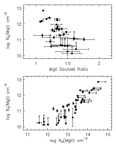
FIG. 5.6 --- The AOD column density of {\MgI} verses the {\MgII} doublet ratio (upper panel) and the AOD {\MgII} column density for individual subsystems.
It is interesting to speculate that the anticorrelation of log N(Mg I) - log N(Mg II) with log N(Mg II), in light of the charge exchange process between H II and Mg I, may be indicating that the gas density, and not the line of sight path length, is governing the Mg II strength. The charge exchange rate is proportional to the product of the H II and Mg I number densities (multiplied by a temperature sensitive reaction coefficient that is the integral over all particle velocities). As such, charge exchange rates in general are sensitive density indicators. If large column density Mg II absorption arises in higher density clouds, it would be expected that the charge exchange between H II and Mg I would be more dominant when N(Mg II) is large and decreasing in importance as N(Mg II) decreases. This charge exchange is a source of ionization for Mg I, so that a trend in its rate would results in trends in the relative abundance of Mg I to Mg II. It is not unreasonable to assume that the strongest absorption arises in regions of peaked over density rather than in more diffuse structures that have line of sight velocity caustics. Rauch, Haehnelt, & Steinmetz (1996) have found that this is indeed the case, that metal-line absorption profiles are most strongly correlated to the density peaks in their simulated structures.
5.2 DOPPLER PARAMETERS
The distribution of Doppler b parameters can provide clues to the thermal and/or dynamical conditions of the absorbing clouds. One unresolved question is whether the internal motions of clouds are predominantly thermal or if there is a significant turbulent or bulk motion component. If the internal motions of a given cloud are predominantly thermal, the b parameter scales as

which results from the square root of the ratio of the ion masses. It is unfortunate that the ratio is not larger, so that a greater leverage can be applied to the problem of deconvolving the relative contributions of thermal and non-thermal line broadening. The technique for this has been described in Section 4.4.3, where it was applied to the simulations. Additionally, if the clouds are predominantly broadened by non-thermal processes, and if the predominant process was correlated with cloud velocity or cloud size, then a correlation between the velocity or the column density and the Doppler parameter might be anticipated.
5.2.1 Distribution of Doppler Parameters
The binned distribution of Mg II, Fe II, and Mg I Doppler b parameters is presented in Figure 5.7. The distribution peaks are ~ 3.5, ~ 5.5, and ~ 4.5 km/s, respectively. Based upon the Blending Simulations, the observed distribution peak could be shifted to a larger value by as much as 2 km/s. The simulations demonstrate that the underlying distribution is probably more highly peaked at a lower b value and does not have as extended a tail. It is also likely that parameters with b < 2 km/s are artifacts of the fitting process (see Figure 4.7 and Figure 4.16.
Figure 5.7
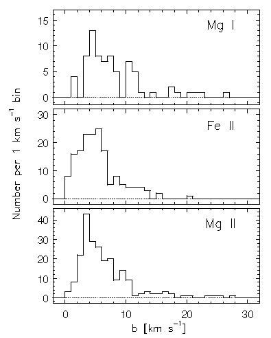
FIG. 5.7 --- The binned distribution of Doppler $b$ parameters for {\MgII} (lower panel), for {\FeII} (center panel), and for {\MgI} (upper panel)
The median of the 148 Mg II parameters included in the sample is 5.0 km/s with a standard deviation of 4.3 km/s, and mean is 6.2 km/s. The distribution skew is 2.0 and the kurtosis is 5.5 (pointier than a normal distribution). Thus, the shape of the distribution differs significantly from a normal distribution in that the skew is a 6-sigma departure and the kurtosis is a 7-sigma departure for a sample this size. The median of the 83 Fe II parameters included in the sample is also 5.0 km/s but with a standard deviation of 2.8 km/s. The mean equals the median. The shape of the distribution is consistent with a normal distribution in that the skew and kurtosis are consistent with zero. The median of the 75 Mg I parameters included in the sample is 6.8 km/s with a standard deviation of 8.2 km/s, and a mean of 8.6 km/s. The distribution skew is 4.3 and the kurtosis is 2.4 (pointier than a normal distribution). Thus, the shape of the distribution differs significantly from a normal distribution in that the skew is a 9-sigma departure for a sample this size. The measured kurtosis, on the other hand, is only a 2-sigma departure.
As the basic statistics dictate, the Mg II and Fe II distributions have quite different shapes, particularly in the range 6 < b < 10 km/s. Given that the parameters were allowed to vary freely between ions for a given component, it is not surprising that the shapes do not closely follow one another. At face value, the different shapes, and the fact that the peak of the Fe II parameters is larger than that of the Mg II, is not suggestive of thermal broadening in the clouds. There is an extended tail in the Mg II distribution that is not present in the Fe II distribution. This may be an artifact of the higher level of constraints placed upon the Fe II in many cases when multiple transitions were available for fitting. When the strong transitions were saturated, the weak transitions were still useful for obtaining well constrained VP parameters. The Mg II transitions, on the other hand, were not as well constrained. The severity of such an effect depends upon both the clustering and the underlying distribution of individual line widths. If the clouds are tightly clustered and have b parameters greater than the average velocity separation, then blending can result in unresolved components in the strongest transitions. On the other hand, if broad and varied profile shapes are governed primarily by the density variations in material with systematic velocities, then the VP decomposition is likely to yield results inconsistent with the simple picture of isolated isothermal clouds.
Petitjean & Bergeron (1990) found a Mg II b distribution peaking at 10 < b < 15~km/s, with a decaying tail at b > 20 km/s. They claim, for the most part, that the individual absorbing clouds have been resolved by the VP profile fits to their 30 km/s resolution spectra. Based upon this finding, they argue that non-thermal or turbulent motions within the individual clouds are implied because such large b values correspond to temperatures in excess of 10^5 K, which implies ionization levels too high for Mg II to survive. In other words, a picture in which the clouds are not quiescent had been inferred. The extended tail in the Mg II parameters, however, should only be taken as evidence of non-thermal motions in as much as the VP decomposition is taken to be an appropriate technique for "measuring" gas properties. Parameters with b > 11 km/s occur, in all cases, within the < 80 km/s velocity range in broad saturated profiles (see Figure 5.12). Thus, they are not well constrained (though their fractional uncertainties are less than unity) nor do they arise in profiles suggestive of being the composition of isolated Voigt profiles.
5.2.2 Inferring the Cloud Temperatures
In Figure 5.8. the Fe II and the Mg I Doppler parameters are plotted verses the Mg II Doppler parameter. Only VP components for which the fractional errors are less than unity are plotted. For the Fe II verses Mg II parameters, the dotted line gives the 1:1 correlation line, the expected relation if the clouds are dominated by non-thermal internal motions. The dash-dot line gives the thermal relation. For the Mg I verses Mg II data, the dotted line gives the 1:1 correlation, expected if the absorption of the neutral component arises in the same spatial region as the ionized component. This plot of b(Fe II) verses b(Mg II) parameters corresponds to Figure 4.8 (lower panel) and to Figure 4.14 (lower panels) presented for the simulations. The input relationship between the Fe II and the Mg I Doppler parameters for those simulations was strictly thermal. Based upon the large scatter that resulted from the simulated VP decompositions, for both the blended and unblended cases, it is clear that the data are not altogether inconsistent with thermal clouds.
Figure 5.8
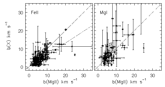
FIG. 5.8 --- The Doppler $b$ parameters of {\FeII} (left panel) and of {\MgI} (right panel) verses those for {\MgII}. Plotted are those data points for which the fractional error is less than unity. The dash--dot line in the left panel is the thermal relationship between {\FeII} and {\MgII} and the dotted line is the 1:1 correlation, which is the non--thermal expectation. The dotted 1:1 correlation line in the right panel is the expected relationship for {\MgI} and {\MgII} co--existing in gas of the same temperature and/or having the same turbulent motions.
The ratio b(Mg II)/b(Fe II) and the ratio b(Mg II)/b(Mg I) are plotted verses component velocity in Figure 5.9. The two lines of constant b(Mg II)/b(Fe II) at 1.0 and 1.53 bracket the range over which physically meaningful cloud properties can be inferred by deconvolving the thermal and non-thermal (turbulent) components of the total Mg II and Fe II b parameters. The line of constant b(Mg II)/b(Mg I)= 1.0 gives the expected value if the neutral absorption arises in the same spatial region as the ionized component. Those components for which b(Mg II)/b(Mg I) > 1 can be inferred to have Mg I absorption arising in gas that is cooler than that in which the Mg II absorption arises. The unlikely opposite case can be inferred when b(Mg II)/b(Mg I) < 1. There is no compelling evidence that the gas temperatures or non-thermal conditions in the neutral and ionized components of the absorbing gas differ. This provides assurance that the assumption applied to the VP decomposition, that the neutral and ionized components were one and the same, is not terribly incorrect.
Figure 5.9
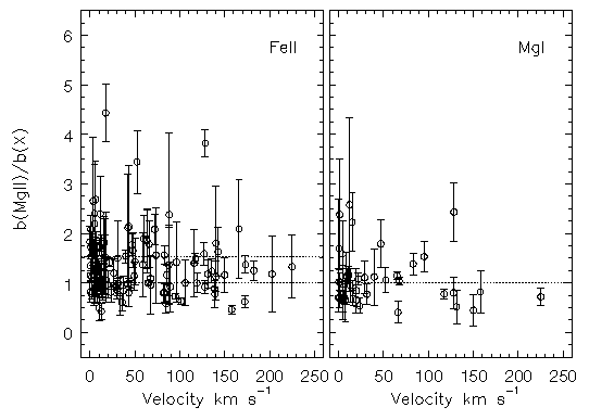
FIG. 5.9 --- The ratio of Doppler $b$ parameters for {\FeII}/{\MgII} (left panel) and for {\MgI}/{\MgII} (right panel). The two dotted lines in the left panel give the range from pure thermal relation (1.53) and pure non--thermal relation (1.00). ``Clouds'' for which physically meaningful temperatures can be inferred must lie within this range. The dotted line in the right panel is the expectation for {\MgI} and {\MgII} co--existing under the same physical conditions. Those components for which $b(\hbox{\MgII})/b(\hbox{\MgI}) > 1$ can be inferred to have {\MgI} absorption arising in gas that is cooler than that in which the {\MgII} absorption arises. The unlikely opposite case can be inferred when $b(\hbox{\MgII})/b(\hbox{\MgI}) < 1$.
In Figure 5.10, the result of deconvolving the thermal component to the line broadening is presented. The selected data have fractional errors less than 20% in both Mg II and Fe II total Doppler b parameters and the plotted curves are lines of constant non-thermal, or turbulent motion. This diagram is the same as Figure 4.9 (lower panel) and Figure 4.15 (lower two panels). As was concluded above, the data are not altogether inconsistent with thermally broadened clouds. The median of the 56 thermal Doppler parameters included in the sample is 4.7 km/s with a standard deviation of 3.5 km/s, and the mean is 6.1 km/s. The distribution skew is 1.2, which is a 2.3-sigma departure from a normal distribution for a sample this size. The kurtosis is consistent with zero. Thus, the distribution is not altogether inconsistent with a normal distribution. The median and mean values correspond to the cloud temperatures T = 32,000 and 54,000 K, respectively. The inferred mean turbulence b parameter can be obtained from

This result, however, is quite uncertain, and does not place useful constraints on the value of the mean non-thermal component in Mg II absorbing clouds.
Figure 5.10
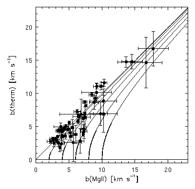
FIG 5.10 --- Deconvolution of the {\MgII} Doppler $b$ parameter, yielding the inferred thermal component of the absorbing clouds. The selected data have fractional errors less than 20\% in both {\MgII} and {\FeII} total Doppler $b$ parameters. The solid curves are lines of constant non--thermal, or turbulent motion.
5.2.3 Are Mg II Clouds Quiescent?
If Mg II absorbing clouds are roughly isothermal across the zones where singly ionized elements are abundant, and the temperatures are more or less independent of the cloud mass, then the expectation is that the inferred temperature of the clouds would be independent of the amount of material the QSO line of sight sampled, i.e.~the column density. As such, no correlation between column density and Doppler parameter should result from the VP decomposition. On the other hand, non-Gaussian features in the optically thick regions of the Mg II profiles may be revealing a far more complicated range of physical states in the gas. A wide range of physical states associated with a single complex absorption profile have been identified in the simulations of high-redshift high-ionization gas (Haehnelt, Steinmetz, & Rauch 1996) and compared to VP decompositions of both simulated spectra and unpublished HIRES/Keck spectra (Rauch, Haehnelt, & Steinmetz 1997). Often, these absorption profiles are sampling only a small over dense region of a large kinematically systematic structure. For example, Rauch, Haehnelt, & Steinmetz suggest that, in principle, a large infalling complex may be identified by broad C IV profile wings across which the gas density and temperature are variable. VP decomposition of such profiles may in fact result in correlations (or anti-correlations) and at the very least result in VP parameters having little in common with the underlying physics of the absorbing gas. Though the physical scale of the C IV systems is larger than that of the Mg II systems, such considerations are most relevant in the case of Mg II absorbing gas when a given system exhibits broad saturated profiles that yield somewhat ambiguous VP decompositions.
Given such considerations, it is of interest to search for correlations between VP column density and Doppler parameters, and in the process, determine if the correlation is an artifact of the VP decomposition itself, or is a true signature from the data. As discussed in Section 4.5.5, it appears that blending in high signal to noise spectra may indeed induce a weak correlation between the column densities and b parameters. It is important to remember that this simulation was of a population of isothermal clouds which did give rise to Voigt profiles in the absorption spectra. Many discussions regarding induced correlations have been addressed in the literature on the Ly-alpha forest (see Khare et al. 1997) and references therein).
In Figure 5.11, the Doppler b parameters are plotted verses the VP column densities for both Mg II and Fe II. The upper panels show all VP components and the lower panels show those with less than unity fractional errors in both b and in log N. The vertical shaded regions give the zone of completeness for the column densities and the horizontal shaded regions give the minimum resolution. Spearman-Kendall tests on these distributions, presented in Table 5.1, reveal no sign of a correlation for the Fe II data with the small fractional errors. However, the Mg II data appear to show strong correlations for both the full sample, P = (2 x 10^-5 , 2 x 10^-6), and the limited sample with small fractional errors, P(0.002, 0.002). For the limited sample, the three data points with N(Mg II) < 11.5 cm^-2 were removed from the test even though they are shown on Figure 5.11. In the case of the Blending Simulations, limiting the correlation test to those data with small fractional errors reduced the the Spearman-Kendall probabilities to the level that any correlation was only suggestive. For the observed data, the correlation persists to a high confidence level, 99.8%. This correlation could arise either as an artifact of the VP decomposition technique, such as the inclusion of small clouds required to obtain a better fit to the spectra, or because the VP decomposition method provides a poor description of gas that is complex and varied in its underlying distributions.
Figure 5.11
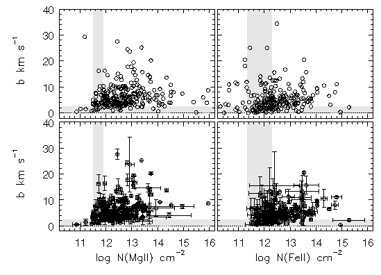
FIG. 5.11 --- The Doppler $b$ parameters verses the VP column densities for {\MgII} (left panel) and for {\FeII} (right panel). The upper panels show all VP components and the lower panels show those with less than unity fractional errors in both $b$ and in $\log N$. The vertical shaded regions give the zone of completeness for the column densities and the horizontal shaded regions give the minimum resolution.
In Figure 5.12, the distribution of Mg II VP columns densities and Doppler b parameters are shown as a function of velocity. It is interesting that, for v > 160 km/s, the b values range between 2 < b < 7 km/s and the column densities range between 11.5 < log N < 12.4 cm^-2, but for the two profiles in the z = 0.8514 system in the Q 0002+051 spectrum. Indeed, one could infer that these clouds are likely to be quiescent, given that their profiles do appear to be well described using VP decomposition. However, these higher velocity clouds may be drawn from a "population" with substantially different physical conditions than those "embedded" in the broad saturated profiles. This is not to imply that all lower velocity clouds are drawn from large gas complexes. It is important to remember the velocity scale is set arbitrarily, and if a given line sight intercepts only a single cloud associated with a larger absorbing complex around a galaxy, this cloud would be given a zero velocity. A good fraction of the Mg II systems have only a single or a few low column density clouds, and they are well described by Voigt profiles. However, if the properties of the gas in these small column density clouds and in these larger absorption "complexes" are not truly different, then one might infer that most all Mg II absorbing gas is quiescent, but that VP decomposition technique breaks down in complex absorption profiles.
Figure 5.12
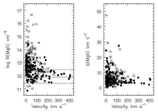
FIG. 5.12 --- The Doppler $b$ parameters verses the VP column densities for {\MgII} (left panel) and for {\FeII} (right panel). The upper panels show all VP components and the lower panels show those with less than unity fractional errors in both $b$ and in $\log N$. The vertical shaded regions give the zone of completeness for the column densities and the horizontal shaded regions give the minimum resolution.
5.3 KINEMATICS
From the work of Sargent, Steidel, & Boksenberg (1988) the two-point correlation function (TPCF) of Mg II systems was known to show a strong peak at Delv < 200 km/s. In 1990, Petitjean & Bergeron found that a two component Gaussian model with sigma_1 = 80 and sigma_2 = 390 km/s provided a good fit to the number of cloud pairs with velocity separations Delv. They observed no systems in the range 700-2000 km/s, which may or may not have affected the result of the broader dispersion. They interpreted the small dispersion to represent clouds bound within galactic halos and the broader dispersion to represent galaxy pairs. They compared the broader component with the correlation of galaxy pairs in clusters, which have too high a dispersion by a factor of two to explain Mg II absorbers separated by these velocity intervals. Mg II absorbing galaxies are mostly identified as field galaxies (Bergeron & Boisse 1991; Steidel 1993a), so one interpretation of the broader component is that it samples galaxy pairs in the field.
Following these authors, the clustering function for Mg II absorbing clouds has been computed. However, the formal TPCF, which includes all clouds from all systems as if they were placed along a single line of sight at their measured redshifts, was not computed. Instead, the "cloud-cloud clustering function" of clouds within systems was computed. Quite simply, the TPCF was computed for each Mg II system and then the result concatenated together into a list of halo cloud velocity separations. Thus, there is no information for velocity scales larger than ~500 km/s. For the following discussion, this will be referred to as the two-point clustering function (also abbreviated TPCF).
In Figure 5.13, the binned TPCF for Sample B (upper panel) and for the subsample of z < 1 systems (lower panel) is presented, where the bin size is 10 km/s. The simplest description of the distributions is that of a superposition of Gaussians. The overall sample exhibits what appears to be two underlying cloud-cloud clustering dispersions, sigma_1 = 30 and sigma_2 = 150 km/s. What is interesting is that the z < 1 subsample shows a slight narrowing in the broader component, sigma_2 = 140 km/s, but is consistent with no change in the narrower component, sigma_1 = 29 km/s. The other notable feature is the relative amplitude of the two components. These effects are likely due to the bias in the equivalent width distribution of systems at high redshift. Since few small EW(rest) systems have been sampled at higher redshift, there are simply fewer small dispersion systems relative to the larger dispersion systems. This likely provides one source for the reduced amplitude in the narrower component. The z > 1 systems are dominated by four EW(rest) > 1.9 A systems. There are no systems in the z < 1 subsample with such large EW(rest). The number density of weak systems is seen to evolve only weakly, if at all, whereas the stronger systems are seen to evolve quite strongly (SS92). In fact, in the large sample of SS92, there are only one or two, such systems at z < 1. The reduced dispersion of the broader component in the TPCF is likely a direct result of removing these four systems from the sample. This would also have the effect of "elevating" the amplitude of the narrow component.
Figure 5.13
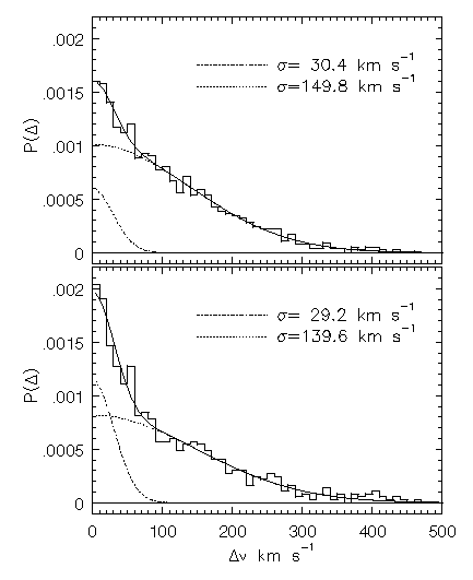
FIG. 5.13 --- The two--point clustering function of VP components within absorbing systems. The upper panel is the full Sample B. The lower panel is for $z_{\rm abs} \leq 1$ systems, which are believed to not be biased in their equivalent width distribution. Both samples required a double Gaussian fit.
A robust measure of how the TPCF evolves, if it does, would require a doubling of the sample size with the goal of obtaining 1 < z < 2 absorbers with an unbiased distribution of EW(rest). Quantification of evolution in the cloud-cloud clustering is key to developing a clear picture of the origins and fates of extended gaseous environments and of their role in structure formation and galaxy evolution.
5.3.2 Modeling the Cloud Kinematics
Motivations for why a disk component is likely to be present within the population of absorbers are given in Charlton & Churchill (1996). Their motivation was based upon cross section arguments (see their Figure 1). At the very least, they were able to demonstrate that randomly oriented extended thick disks with reasonable aspect ratios present a geometric cross section that is competitive with spherical halos. However, the object of the work presented here is to examine how well a given kinematic model can give rise to absorption properties that match the observed ones. For that reason, it is instructive to examine extreme, yet simple, models. Here, we consider a population of rotating disks, a population of spherical infall halos, and a population of hybrid disk and infall halos. The following is based upon the current work of Charlton & Churchill (1998).
5.3.2.1 Design of the Disk (D) Model
The disk shape, seen edge-on, can be likened to a bow tie. The inner 10 kpc has a thickness of z = 1 kpc. The disk extends to

while the thickness outward from R > 10 kpc in radius increases to the maximum thickness of z = 10 kpc. The R(L_B) scaling is taken from Steidel (1995). The factor 1.5 accounts for the cut off of the extended disk (see Charlton & Churchill 1996), though the absorption properties of the disk are not sensitive to the exact value. The rotation curve is solid body out to R = 5 kpc and then is flat beyond that point based upon the Tully-Fisher relation,

where v = 200 km/s has been assumed for an L* galaxy. The galaxy luminosity is selected from a Schechter function,

with alpha = -1.0 (see Charlton & Churchill 1996). The z direction dispersion of the clouds was varied and a final value of 15 km/s was adopted because it provided the best match to the observed TPCF. The individual, randomly placed clouds have sizes r_cl = 1 kpc.
5.3.2.2 Design of the Infall Halo (IH) Model
For the Infall Halo Model, the clouds are distributed randomly in a sphere of radius

where the R(L_B) scaling is taken from Steidel (1995). The cloud velocities are purely radial and directed toward the sphere center with magnitude

where v = 200 km/s has been assumed for an L* galaxy. As with the disks, the galaxy luminosities are selected from the Schechter function. Unlike the disk, which incorporated random motions in the z direction, there are no random motions introduced to the cloud velocities. In Figure 5.14, a sample of 50 synthetic spectra from the IH model are presented with the VP decompositions and model spectra (see below).
Figure 5.14
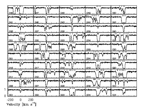
FIG. 5.14 --- A grid of 50 {\MgII} $\lambda 2796$ transitions and the {\minfit} model for the Infall Halo (IH) model.
Figure 5.15
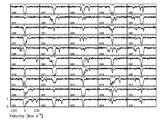
FIG. 5.15 --- A grid of 50 {\MgII} $\lambda 2796$ transitions and the {\minfit} model for the D+IH Model. A cutoff of $\log N(\hbox{\MgII}) = 12.5$~{\cm2} has been applied as the maximum column density for the halo clouds.
The generation of synthetic absorption spectra follows closely the procedures discussed in Chapter 4, once a table of cloud properties and velocities are in hand for a given line of sight through the modeled absorbing structure. The number of clouds and their velocities are determined by searching along the random line of sight through the absorber, which means that the spatial location and local velocity within the model structure must be known at each location along the line of sight. For the disks, the procedure is somewhat complicated by the fact that they are randomly oriented in a three dimensional coordinate system. A rotation matrix is used for the coordinate transform and for the computation of the projected line of sight velocity.
For each entry in the resulting list of intercepted clouds, the column density and Doppler b parameter is selected from distribution functions. The N(Mg II) distribution is a power law with slope delta = 1.57 with lower and upper cutoffs of 11.5 < log N(Mg II) < 15.5. The Doppler b parameters are selected from the list of observed parameters. The N(Fe II) are given by the same relation used for Simulation 2 (see Equation~\ref{eq:columnrat}) and the b(Fe II) are given by the thermal relationship between Doppler b parameters (see Equation~\ref{eq:thermalb}). Once the list of Mg II and Fe II cloud column densities, Doppler parameters and velocities are in hand, the synthetic absorption spectra are generated following the procedure described in Section 4.1. The spectra were then analyzed using the identical procedures used on the HIRES spectra.
Each spectrum was given a signal to noise ratio of ~30 per resolution element. This corresponds to a 5-sigma equivalent width detection limit of 0.013 A. Though the number of VP components was found to be sensitive to the signal to noise ratio of the spectra, the number of kinematic subsystems (subfeatures identified by ewregion) were not (see Table 3.4). The subsystem analysis, as presented in Chapter 3, turns out to provide useful constraints on the acceptable model parameters (once the general kinematic model is adopted). It turns out that the TPCF provides the strongest constraints on the parameters used to describe basic kinematics in the context of a simple rotating disk and infall halo model. A series of models were designed and analyzed. The analysis consisted of attempting to match the observed TPCF, and the velocity distributions of subsystem equivalent widths, velocity widths, asymmetries, and doublet ratios.
In Figure 5.16, the TPCFs for the disk model and the infall halo model are shown in the upper two panels. The infall halo model required a two component Gaussian fit. The disk model produces a single component Gaussian TPCF, and it is pretty clear that it fails as a single population absorber. It was thought that the two component Gaussian shape to the infall halo TPCF may be due to the functional dependence the cloud velocities on the galaxy luminosity. However, when a single population of L* galaxies were used for the infall halo model, the two component Gaussian remained virtually unchanged. This result is quite surprising and interesting. A single kinematic population can give rise to what appears to be two populations. The need to fit multiple Gaussian components to a TPCF does not necessarily imply more than one population of absorber kinematics nor does it imply a distribution of a single population of absorber kinematics.
Figure 5.16
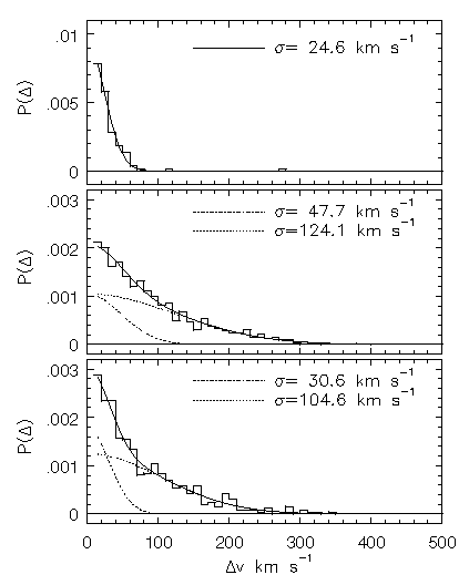
FIG. 5.16 --- The two--point clustering function (TPCF) of three kinematic models. The disk model is well fit by a single Gaussian, whereas the halo model requires a two Gaussian fit. The D+IH model also requires a two Gaussian fit.
Based upon these TPCFs (and inspection of the velocity distributions of the subsystem absorption properties), it became clear that a "hybrid" disk and infall halo model should be examined. The disk plus infall halo (D + IH) model is simply a combination of the disk model and the infall halo model. In Figure 5.15, simulated spectra of the Mg II 2796 transition are shown for 50 realizations. Several trial cases were run and analyzed.
5.3.2.4 Comparing to Observations
A good match to the observed TPCF was obtained when the z velocity dispersion in the disk was set to 15 km/s, as shown in the lower panel of Figure 5.16. The shape and decomposition of the TPCF, particularly the narrow dispersion component, was quite sensitive to this parameter. Varying its value by +/- 5 km/s resulted in a change of +/- 10 km/s in the narrow component, sigma_1. The other artifact was the relative amplitudes of the two Gaussian components. The TPCF presented for the D + IH model is consistent with the observed TPCF within the uncertainties of the Gaussian parameters.
The observational data most challenging to reproduce are those presented in Figure 3.8 and Figure 3.11. Specifically, these are the subsystem absorption properties as a function of velocity and the distribution of these properties for the v < 40 km/s and v > 40 km/s populations of the subsystems, respectively. It turns out that breaking the absorption systems into subsystems, defined as subfeatures using ewregion, provides a powerful diagnostic for the kinematic models. The challenge is to reproduce the distribution of these absorption properties for the overall system and for the subsystems.
In Figure 5.17, the subsystem equivalent widths, EW(rest), and velocity widths, omega_v, are presented as a function of velocity for two D + IH models . Their observed distributions provide tight constraints on the overall morphology of the absorption profiles. As discussed in Section 3.4.3, roughly 80% of v > 40 km/s subsystems account for subsystems with EW(rest) < 0.2 A. Moreover, all of the v >40 km/s subsystems have omega_v < 20 km/s, with 85% of them having omega_v < 10 km/s. Taken together, these results are suggestive that these subsystems are a subpopulation characterized first and foremost by their velocity with respect to the optical depth mean of the overall system. These clouds appear to constitute a population that may be spatially distinct from the main absorbing complex in the system. If so, they may be subject to environmental conditions that limit their sizes, densities, and or temperatures.
Figure 5.17
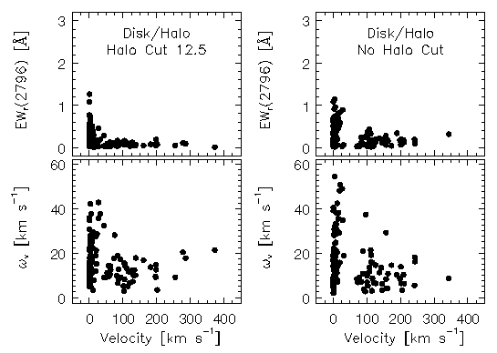
FIG. 5.17 --- Subfeature absorption properties verses velocity for models D+IH 1 (left panels) and D+IH 2 (right panels). Presented are the equivalent width (upper panels) and the velocity width (lower panels). These distributions are to be compared to the observed distributions in Figure~\ref{fig:allvsvel} (also see Figures~\ref{fig:subfeatvbin} and \ref{fig:assorted1hiv}).
The following results are very preliminary, based upon applying a cutoff in the upper column density of clouds in the infall halo component to the D + IH model. An upper cutoff of log N(Mg II) = 12.5 cm^-2 was applied. Such a cutoff might be understood if clouds distributed in the halo were not shielded to ionizing photons due to their lack of proximity to other larger clouds. A cutoff of log N(Mg II) = 12.5 cm^-2 corresponds to a log N(H I) ~ 17.3 cm^-2 cloud. The implication would be that halo clouds arise in optically thin material. The effects of applying this cutoff are illustrated in Figure 5.17, Figure 5.18, Figure 5.19.
Figure 5.18
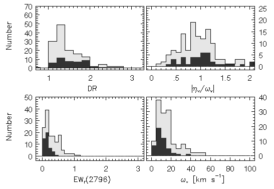
FIG. 5.18 --- Based upon the subfeature velocity distribution of the observational data (see Figure~\ref{fig:subfeatvbin}), the properties of subfeatures with $v>40$~{\kms} were binned as a separate population of absorbers --- (upper left) the doublet ratios --- (lower left) the equivalent widths --- (upper right) the subfeature asymmetries per unit width (shape parameter) --- (lower right) the subfeature velocity widths. The lightly shaded histograms are all subfeatures (all velocities) and the solid filled histograms are the $v>40$~{\kms} sub--population. This figure is to be compared to Figure~\ref{fig:assorted1hiv} (observed data) and to Figure~\ref{fig:assorted_cutoff}.
The left panels of Figure 5.17 show model D + IH 1, for which the column density cutoff has been applied and the right panels show model D + IH 2, with no cutoff. One hundred realizations of each model are presented. Compared to the observed data, they both fail to reproduce the very narrow velocity widths. As seen in Figure 5.18 and Figure 5.19, the distributions, the velocity widths of all subsystems, even those at v < 40 km/s, are too wide (the omega_v < 5 km/s bin is relatively empty). However, the equivalent width distributions are a better match to the data for model D + IH 1. As seen in Figure 5.19, the distributions of doublet ratios are in fair agreement with those observed. On the other hand, the doublet ratios for model D + IH 2 show no dependence on the velocity; there are as many v > 40 km/s subsystems in the flat part of the curve of growth as on the linear part, which is not seen for the data.
Figure 5.19
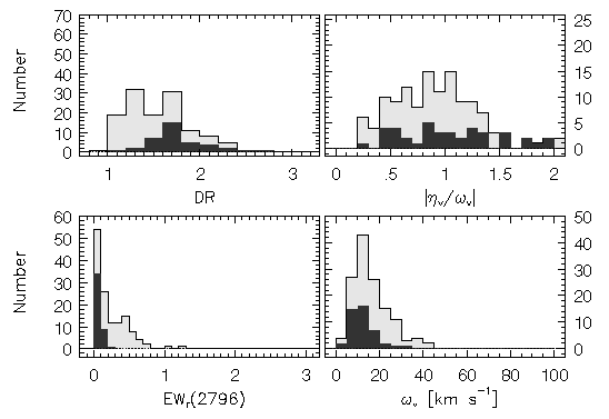
FIG. 5.19 --- Model D+IH 1. Based upon the subfeature velocity distribution of the observational data (see Figure~\ref{fig:subfeatvbin}), the properties of subfeatures with $v>40$~{\kms} were binned as a separate population of absorbers --- (upper left) the doublet ratios --- (lower left) the equivalent widths --- (upper right) the subfeature asymmetries per unit width (shape parameter) --- (lower right) the subfeature velocity widths. The lightly shaded histograms are all subfeatures (all velocities) and the solid filled histograms are the $v>40$~{\kms} sub--population. This figure is to be compared to Figure~\ref{fig:assorted1hiv} (observed data) and to Figure~\ref{fig:assorted_nocut}.
It could be that tuning the Doppler b distribution may bring the distribution of velocity widths into better agreement with the data. For the optically thin halo clouds, the b distribution could be peaked well below the average found for the observed data. This would reduce the velocity widths, but would presumably not have as large effect on the equivalent widths, since they are independent of b on the linear part of the curve of growth. Drawing the b parameters from the observed distribution is not the appropriate approach. This is further exemplified by the center panels of Figure 5.20. The b distribution input to the models is shown with the thick line histogram and the resulting out from the VP decomposition of the simulated spectra are shown with the thin line histogram. The upper panel is model D + IH 1 and the lower panel is model D + IH 2. The vertical axes are arbitrary number per bin. The output distribution is not consistent with having been drawn from the input distribution.
When the b distribution of both the disk and the halo components are drawn from a Gaussian with b = 3.5 km/s and sigma_b = 2.0 km/s with b_cut = 2.5 km/s, the TPCF is highly peaked relative to the observed TPCF. The narrow Gaussian component has sigma_1 = 14 km/s, compared to the observed 30 km/s. Further investigation of the available parameter space is studied by Charlton & Churchill (1998).
Figure 5.20
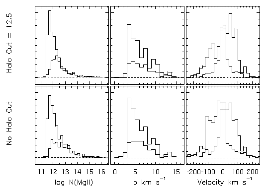
FIG. 5.20 --- The distribution of {\MgII} VP column densities (left panels), Doppler $b$ parameters (center panels), and VP component velocities for models D+HI 1 (upper panels) and 2 (lower panels). The thick histograms are the input data (see text) and the thin histograms are the resulting VP parameters. Note that the incompleteness in the $\log N$ distribution is sensitive to the halo cloud column density cutoff, but that the distribution at higher $\log N$ is well recovered. Also note how assigning a velocity zero point to the profiles dramatically changes the component velocity distribution.
The preliminary conclusions that can be reached based upon the current level of exploration of model parameters, is that
- A multi-component Gaussian decomposition of the TPCF does not
necessarily imply that the absorbing clouds are comprised of
more than one type of systematic kinematics.
- It is not trivial to recover the observed values of the TPCF
Gaussian components, which have placed a fairly tight constraint on
the z dispersion of the disk material.
- Some combination of extended thick disk plus infall halo
provides a promising model in that its simple kinematics yield a
TPCF with Gaussian components consistent with those describing the
observed TPCF.
- Using an upper limit to the cloud column density in the infall halo component goes a long way toward reproducing the distribution of equivalent widths and doublet ratios of the v > 40 km/s subsystems.
5.3.2.5 Information Lost: Models Lessons
The data in Figure 5.20 reveal the added benefit of the analysis technique applied to the kinematic models. In the left hand panels, the distribution of column densities is presented for the input (thick histogram) and for those resulting from VP decomposition (thin histogram). The input power law is well recovered to log N(Mg II) ~ 13 cm^-2 for model D + IH 2. The onset of incompleteness at such a high column density is not consistent with the observed data, which have an onset of incompleteness at N(Mg II) ~ 12.5 cm^-2. Interestingly, model D + IH 1, with the upper column density cutoff in the halo component recovers this incompleteness threshold. The redistribution of column densities and the threshold of completeness is model dependent, which means that it too offers a constraint and a tool for insight.
The right panels in Figure 5.20 give a powerful illustration of how the underlying cloud velocities intercepted by the line sight are distributed with respect to the galaxy itself. More profoundly, it illustrates how using the optical depth median to reset the velocity zero point redistributes the clouds. As with the other quantities, the thick histogram is the model input data and the thin histogram is the data resulting from the VP decomposition of the simulated spectra. The reduced area under the thin histogram gives the number of input clouds lost through the analysis.
The bottom line is that the models appear to be well constrained by the observational data. If the tuning of disk and halo model parameters each have a somewhat unique manifestation in the output VP components, TPCF, and subsystem absorption properties, then the present line of analysis holds the promise of revealing a great deal of insight into the spatial and kinematic distributions of absorbing gas in galaxies. Clearly more experimentation is needed, given the preliminary level of the presented analysis.