4. ASSESSING VP DECOMPOSITION OF HIRES SPECTRA
One of the motivational factors for decomposing high signal to noise high resolution absorption lines into Voigt profiles is the promise that the chemical, ionization, and internal physical conditions in individual absorbing clouds might be inferred. Since the VP decomposition of absorption features yields only parameterized quantities that are a function of the VP fitting philosophy, it is not clear that the gas properties are being represented accurately. In other words, it is not clear to what level VP decomposition fitted parameters reflect the "true" cloud properties even in the case where they are known a priori .
In order to examine the level at which inferences can be drawn from the minfit VP results, simulations were run in which spectra of the Mg II 2796, 2803 doublets and the five Fe II transitions in Table 2.1 were fit with VP components. Similar simulations have been undertaken by Lu et al. (1996a) and by Hu et al. (1995) for the Ly-alpha forest. These groups found that line blending resulted in an artificial roll over in the column density distribution at low column densities when a power-law distribution was used to generate the synthetic absorption line spectra. The significant difference between the simulation performed here and those for the Ly-alpha forest are that (1) the hydrogen absorption-selected clouds were assumed to be distributed cosmologically, whereas the Mg II absorbing clouds are clustered in kinematic systems, and (2) the VP decompositions of the Mg II systems included simultaneous fitting to the Mg II doublet and, for some simulations, to five Fe II transitions as well.
There are five basic categories of questions that address the degree to which known input parameters are recovered from the VP parameterization of absorption features.
-
What is the column density detection limit for a sample of single
component Mg II doublet transitions for spectra with a well
defined rest-frame equivalent width detection limit?
What are the Fe II and Mg I column density detection limits?
This knowledge is central to understanding the effects of partial
completeness when the spectroscopic sample is comprised of a finite
range of rest-frame equivalent width detection limits.
-
How does simultaneous VP decomposition of the Fe II
transitions influence the resulting VP parameters for single
component Mg II doublet transitions?
Do Mg II VP parameters change in any fundamental or systematic
way based upon constraints provided by simultaneously fitting
Fe II profiles, particularly in the regime where Mg II
is saturated?
-
How sensitive are the minfit results to the initial VP model
as obtained using autovp and/or profit in the
case of single component profiles?
This is a question of uniqueness for the overall VP fitting
procedure, and can be addressed by using the VP parameters used
to generate the simulated absorption lines as the initial model
for minfit.
-
To what degree of accuracy can the presence of turbulent
(i.e. non-thermal) broadening of absorption lines be inferred by
comparing the Mg II and Fe II VP Doppler parameters and their
distributions in single component absorption lines?
If pure thermal clouds are simulated, what is the distribution of
the inferred turbulent broadening component and how well are
the cloud temperatures recovered using VP parameterization?
- To what degree does line blending in complex profiles bias the value at which the column density detection limit is complete and how is the inferred distribution of column densities influenced with respect to the known input distribution? Ultimately, how well can the distribution of input column densities be recovered and can a correction be applied to the observational results? How well do the inferred Doppler b and velocity distributions compare to the input distributions? Are statistical correlations in the VP parameters artifacts of the fitting procedure?
Four single component simulations and one blending simulation were carried out to address the above categorized questions, respectively. For each of the single component simulations, 500-2000 HIRES/Keck "spectra" of unblended single VP absorption lines were generated of the Mg II doublet.
For Sample B, the upper equivalent width detection threshold is 0.020 A, which defines the threshold at which the quantities derived from the HIRES data constitute a complete sample. The lowest detection threshold in Sample B is 0.008 A. Thus, 0.008-0.020 A constitutes the range over which some level of "partial" completeness in the number of VP components and parameters occurs. In order to better understand the effects of partial completeness, simulations for these extreme detection thresholds (one full set of simulations for 0.020 A and one full set for 0.008 A) were carried out.
4.1 GENERATION OF THE SIMULATED SPECTRA
For each simulated HIRES spectrum the "absorbing cloud" VP parameters were drawn from empirical distribution functions (based upon preliminary VP analysis of the observational data). Each "continuum normalized" absorption profile was convolved with the HIRES/Keck instrumental spread function (a Gaussian of width 2.46 km/s), following which noise was added. The noise was introduced to each pixel by drawing a random deviate from a Gaussian distribution of width sigma(lambda). The normalized "noise" spectrum was computed from

where F(lambda) is the normalized flux in the pixel centered on lambda, and I_c is the "continuum level" given by

where SNR is the signal to noise ratio per pixel in the continuum chosen to give the desired equivalent width detection limit, and RN=4.3 is the HIRES read noise in electrons. This relation, based upon Poisson photon fluctuations and read noise added in quadrature, allows a realistic reduction of noise in deep line cores with the lower limit given by the read noise itself. The SNR per pixel is determined from

where N_pix = 7 is the number of pixels used for the equivalent width detection limit sigma(EW) at the N-sigma = 5 significance level, and lambda_o is the transition wavelength. The velocity spread per pixel is Delv_pix = 2.058 km/s. These numbers are consistent with those used for feature identification in the HIRES spectra using ewregion. A consistency check was performed by analyzing the simulated spectra with the same algorithms used to analyze the HIRES spectra to establish that simulated spectra did in fact yield the input equivalent width detection threshold.
4.1.1 VP Component Selection Criteria for Analysis
Before embarking upon an analysis of the VP parameters obtained by minfit, it is important to establish the selection criteria by which components will be included for the use of statistics. Moreover, the selection criteria can be different for the different statistical tests. What is deemed most important, is that the VP parameters are statistically complete or are sound components in that they have fractional errors smaller than some defined value.
For a study of the distribution of column densities, it is critical that the analyzed sample is complete to some lower cutoff. Thus, when studying the relationship between column densities of various ions and their column density distributions, only VP clouds with column densities above the completeness threshold for the given equivalent width limit of a particular simulation will be included. When studying the Doppler b parameter distribution and the relationships between column densities and b parameters, it is also important that the VP parameters are well determined. Thus, only components for which the fractional error in both the column density and the Doppler b parameter are less than unity will be included in these analyses. For studies of the velocity distribution, it is important to include the entire sample resulting from the VP decomposition.
These selection criteria are the same as those applied to the VP components obtained for the HIRES spectra.
4.2 SIMULATION 1A: COLUMN DENSITY COMPLETENESS
The purpose of Sim-1A was, for single component lines, (1) to determine the Mg II, Fe II, and Mg I column density detection limits as a function of the rest-frame equivalent width detection limit, and (2) to ascertain the probability of recovering an Mg II input column density as a function of column density. For this, 500 simulated spectra each with fixed column densities at half decade intervals over the range 12.0 < log N(MgII) < 15.5 cm^-2 were generated and features were identified using ewregion. The simulated spectra were then VP decomposed using autovp and minfit. For log N(MgII) < 12.0 cm^-2, the column density "resolution" was increased to 0.1 dex in order to obtain a fairly robust measure of the lower-limit detectable column density. Similarly, the column resolution was set to 0.05 dex for both the Fe II and Mg I detection threshold simulations. The Doppler b parameters were selected from a Gaussian distribution function with mean b = 4.9 km/s, width sigma_b = 1.5 km/s, and lower-end cutoff b_min = 3.0 km/s. This distribution function was selected based upon preliminary fitting to the HIRES spectra (Churchill 1997).
In Figure 4.1, the first five realizations of the Mg II 2796 transition for eight column densities, 12.0 < log N(MgII) < 15.5 cm^-2, are illustrated in order of increasing Doppler b parameter. The minfit models and the number of components are also shown. The full grid would extend rightward another 495 entries. Note that the random seed is the same for the different column densities at each grid number, which explains why the patterns in the noise are common for all column densities. Note that two of the log N(MgII) = 15.5 cm^-2 have been fit by two components. There is a propensity for large-b parameter large-N transitions to be fit by multiple VP components.
Figure 4.1
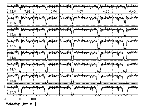
FIG. 4.1 --- A grid of the Mg II 2796 transition and the minfit model for the first five simulations (varying b parameter) for 12.0 < log N(MgII) < 15.5 cm^-2. For presentation purposes, the systems have been order by increasing b parameter, which appears in the lower right corner across the top panels. The column density appears in the lower left corner of the leftmost panels.
4.2.1 The Lower-Limit Detectable Column Densities
In Figure 4.2, the fraction of single component lines detected out of 500 simulated spectra are shown. The solid line gives the relative probability of detecting a single component Mg II absorption doublet. These simulations show that the lower limit Mg II column completeness of Sample B is log N(MgII) = 11.9 cm^-2 to the 99% detection fraction. The dotted line shows that the lower Mg II column density limit detectable in the highest signal to noise HIRES spectrum is log N(MgII) = 11.5 cm^-2. The range between these lines is the region of partial completeness for Sample B. For large N(MgII), autovp often found multiple VP components even though the input model was a single component. In many of these cases, minfit did not eliminate the multiple components handed to it as the initial VP model. The badness parameter was set to 1.5 and the confidence parameter was set to 0.97, to be consistent with the fitting of the HIRES data.
Figure 4.2
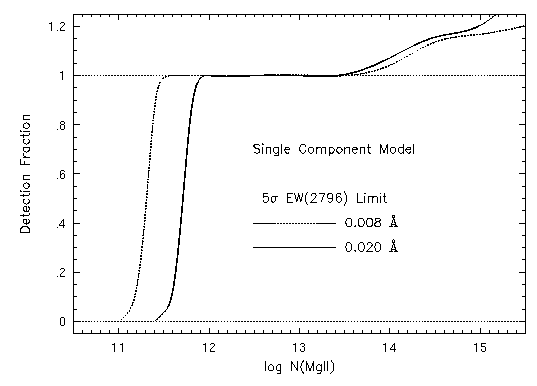
FIG. 4.2 --- The fraction of detected VP parameterized single component Mg II doublets in simulated HIRES spectra. The detection criterion was a 5-sigma significance level in the equivalent width of the Mg II 2796 transition. The solid line, representing Sample B completeness, shows that the completeness lower cutoff is log N(MgII) = 11.9 cm^-2 to the 99% detection level. The dotted line shows that the limit at which partial completeness ends is log N(MgII) = 11.5 cm^-12. At log N(MgII) > 13.5 cm^-2, the detection fraction is greater than unity because multiple VP components are found using autovp and minfit.
The relative detection probability curves for Fe II and Mg I exhibit identical behaviors as shown for the Mg II transitions, and thus are not shown. The lower limit Fe II column completeness of Sample B is log N(FeII) = 12.30 cm^-2 to the 99% detection fraction, and for Mg I is log N(MgI) = 11.45 cm^-2 . The completeness lower limits are log N(FeII) = 11.85 cm^-2 and log N(MgI) = 11.05 cm^-2, respectively. These numbers are predictable to a fair accuracy, once the Mg II limiting column density is established, by equating the optical depths in the optically thin line cores of the respective transitions to that of the line core of Mg II 2796 at its limiting column density,

which can be written,

for log N(MgII) = 11.9 cm^-2 when the transition wavelengths are given in units of A. This simplistic technique yields the predicted limiting column densities of log N(FeII) = 12.4 cm^-2 and log N(MgI) = 11.4 cm^-2, respectively, which are comparable to the simulation results.
4.4.2 Recovering Input Mg II Column Densities
In Figure 4.3, the normalized distributions of the minfit VP column densities to the Sim-1A spectra are shown for both the 0.008 A and 0.02 A equivalent width limits. In the regime log N(MgII) < 13.5 cm^-2, the input column density is recovered to a high probability. However, as the input column density is increased above this value, the probability distribution becomes spread out, and is as broad as an entire decade at the 50% level for log N(MgII) = 14.5 cm^-2 for the 0.02 A limit case. As can be inferred from Figure 4.2, this spread arises because multiple components are fit to the single input component. This trend results in a bimodal distribution for log N(MgII) = 15.5 cm^-2, which is not as severe for the 0.008 A limit case. A naive implication of this result is that, had the input column densities been drawn from a power law number density distribution, the "measured" distribution of column densities would exhibit a paucity of high column density lines relative to the input distribution. Ultimately, the measured distribution function is a convolution of the fitted distribution at each input column density. It is not clear what the magnitude and trend would be in the measured distribution due to the observed broadening and bimodality for saturated profiles. Simulation 2 will be used to address this issue in more detail.
Figure 4.3
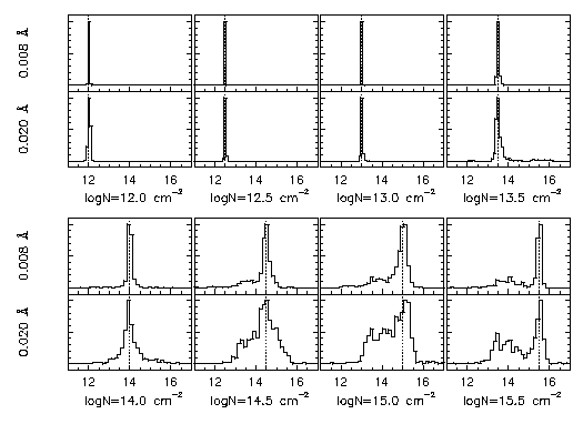
FIG. 4.3 --- The distribution of minfit VP Mg II column densities as a function of the input column density for single component Mg II doublets in 500 simulated HIRES spectra (Sim-1A). The vertical dashed line in each panel gives the input column density (also labeled below the panels). The upper partial panels are for a limiting equivalent width of 0.008 A and the lower are for 0.02 A. Each distribution has been normalized to unity at its peak value.
4.3 SIMULATIONS 1B AND 1C: MODELING SENSITIVITY
The purpose of Sim-1B was to determine if the autovp - minfit processing may be introducing a systematic bias in the resulting VP parameterization of the data. For this Sim-1A was duplicated, except that the autovp step was by-passed and instead the column density and b parameter which generated each simulated Mg II doublet was handed to minfit as the initial model.
The purpose of Sim-1C was to ascertain, for single component lines, how sensitive the probability of recovering an Mg II input column density is to the simultaneous fitting of several Fe II transitions. For example, in the cases where autovp feeds a multiple component VP model to minfit (even though a single component was used to generate the simulated spectrum), do Fe II transitions influence the minfit algorithm in a systematic way to reject the multiple components and yield only a single component? For this, 500 simulated spectra each with fixed column densities at half decade intervals over the range 12.0 < log N(MgII) < 15.5 cm^-2 were generated and the features were identified using ewregion. The simulated spectra were then VP parameterized using autovp and minfit. The relation

was assumed based upon preliminary fitting of the observed Fe II and Mg II column densities (see Section 5.1.1). The Mg II Doppler b parameters were selected from the same Gaussian distribution function used for Sims-1A and 1B. The Fe II Doppler b parameters were computed from the thermal broadening relation,

where m is the atomic mass of the respective elements. The Mg II doublet is saturated for log N(MgII) > 13.5 cm^-2, so that this is the column density regime where the minfit results are expected to be affected.
In Figure 4.4, the normalized distributions of the minfit VP column densities to the Sim-1B and Sim-1C spectra are shown for both the 0.008 A and 0.02 A equivalent width limits. The main result here is two-fold: (1) The trend toward bimodality at large input Mg II column densities is not present, as must be the case. However, the distribution broadening for log N(MgII) < 15.0 cm^-2 is virtually identical as for Sim-1A and 1C. This fact, and the fact that the distribution width for a given input column density increases with limiting equivalent width, suggests that the broadening is an artifact of the signal to noise ratio of the spectra. (2) The inclusion of Fe II does not place a strong constraint on the number of VP components, even though the weaker Fe II transitions are not saturated and are clearly single components. The reason that minfit still retains the multiple components in many cases is because it attempts to reduced the number of components (F-test, see Section 2.6) only when the fractional uncertainties in the VP parameters for the Mg II doublet are greater than the user defined badness parameter (the reference ion for these simulations was Mg II).
Figure 4.4
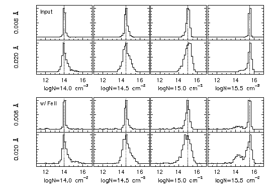
FIG. 4.4 --- The distribution of minfit}VP Mg II column densities as a function of the input column density for single component Mg II doublets in 500 simulated HIRES spectra (Sim-1B and 1C). The vertical dashed line in each panel gives the input column density (also labeled below the panels). The top four panel are from Sim-1B, for which the input VP model parameters were handed to minfit, and the bottom four panels are from Sim-1C, for which five Fe II transitions were simultaneously fit with the Mg II doublet. The upper partial panels are for a limiting equivalent width of 0.008 A and the lower are for 0.02 A. Each distribution has been normalized to unity at its peak value.
It was thought that simultaneous fitting to Fe II transitions would result in multiple VP components that were "bunched" on top of one another in velocity space, following which minfit would then perform an F-test due to overlapping components. However, the "extraneous" VP component was often well constrained by a noise induced asymmetric wing of an absorption profile so that its VP parameters had acceptable fractional errors. The real virtue of simultaneously fitting to Fe II transitions is apparent when multiple and blended profiles are VP decomposed. In these cases, the cloud velocities are well constrained by the weaker Fe II transitions.
4.4 SIMULATION 2: N AND b DISTRIBUTIONS
One purpose of Sim-2 was to determine the degree to which turbulent broadening in the single component "absorbing clouds" can be inferred from a sample of HIRES spectra with a well defined rest-frame equivalent width detection limit. Also, it is important to ascertain if any systematic as a function of input Mg II column density is present in the measured column density distribution, due either to detection limits or saturation when blending effects are known not to play a role. For this, 4000 simulated spectra were generated and for each the input Doppler b parameters were drawn from the distributions used for Sim-1. The Mg II column densities were drawn from the empirically determined power-law distribution function,

which is based upon preliminary fitting of the HIRES spectra (see Section 5.1.1). The column density distribution was taken over the finite region 11.5 < log N(MgII) < 15.5 cm^-2. The lower cutoff corresponds to the completeness limit of the highest signal to noise spectrum in Sample B. The upper limit is rather artificial, and may not necessarily be more appropriate than no upper cutoff. Its inclusion allows an investigation of the number of very large column density clouds resulting from the fitting process. The ratio of Fe II to Mg II column densities was the same as used for Sim-1C. Since the absorbing clouds are assumed to be strictly thermally broadened, it will be straight forward to assess the degree to which turbulent broadening is falsely inferred from the VP parameterizations.
4.4.1 Recovering Input VP Parameters
Accurate recovery of the input VP parameters serves to demonstrate that the minfit algorithm is functioning properly and to provide quantifiable discrepancies between the a priori cloud properties and those inferred from the VP decomposition.
In Figure 4.5, the minfit column densities and Doppler b parameters are plotted against their respective input parameters. For the most part, it can be seen that Mg II column densities are well recovered until the doublet becomes saturated at N(MgII) > 13.5 cm^-2. This is consistent with the results of Sim-1C, in which multiple VP components are sometimes fit to the single component input. The Mg II b parameters follow the correlation line, but with an RMS scatter of ~1 km/s. The Fe II column densities are well recovered over the full input range above the detection threshold of N(FeII) > 12.4 cm^-2. Below this value, the distribution of column densities suffers incompleteness. As illustrated somewhat dramatically by the large scatter in the minfit b parameters for log N(FeII) < 12.5 cm^-2, it is clear that the b parameter is less constrained in weak lines than is the column density.
Figure 4.5
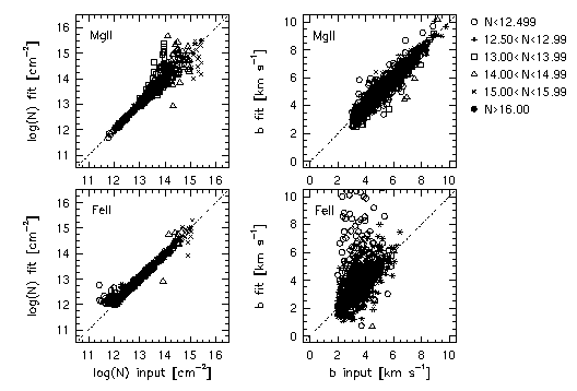
FIG. 4.5 --- The resulting minfit VP column densities and Doppler b parameters for Mg II (upper two panels) and Fe II (lower two panels). The legend to the upper right provides a key to the input VP column densities. The dashed lines show a 1:1 correlation between fitted and input parameters. The formal error bars are not shown for presentation purposes.
Few VP components with 11.5 < log N(MgII) < 11.9 cm^-2 met the selection criteria for inclusion in the analysis even though these column densities are the most abundant in number for the simulation input. This is due to (1) the detection threshold of the Mg II column density, log N(MgII) < 11.9 cm^-2, and (2) the fractional error constraint on the Fe II parameters, since Fe II features have large errors in their VP parameters below the completion threshold for Mg II.
The distributions of minfit column densities for both Mg II and Fe II are illustrated in Figure 4.6. The column densities were fit using the maximum likelihood method (see Section 5.1.1). Since an upper cutoff column density was enforced on the input distribution, the maximum likelihood method was normalized to the observed range of minfit column densities. The minfit column densities have been binned for display purposes only. These data include the full range of detected column densities, not just those above the completeness thresholds. This is to illustrate the incompleteness in VP components, as can be seen in the turnover at small columns. The maximum likelihood fit to the power law function, however, was performed on the unbinned data and included all column densities above the completeness threshold.
Figure 4.6
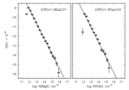
FIG. 4.6 --- The distribution of column densities, f = CN^-delta, output by minfit. The left panel is the Mg II distribution and the right panel is the Fe II distribution. The solid line in each panel is the Sim-2 input distribution and the dashed line is the maximum likelihood fit to the minfit results normalized over the spread of the data (see text). The fit included column densities above the completeness limit for each ion. The fitted power and its uncertainty is given in each panel. For presentation purposes only, the data have been binned at Delta logN = 0.25.
The degree to which the column density distribution is recovered is remarkable in view of fact that the FWHM of the probability distribution for recovering an input column density of log N(MgII) > 14.5 cm^-2 is a full dex (see Figure 4.4). The maximum likelihood power law slope was found to be delta = 1.60 +/- 0.01 for Mg II and delta = 1.65 +/- 0.03 for Fe II, which are roughly 1.5-sigma from the input, delta = 1.57. From the binned data in Figure 4.6, it is apparent that the two maximum likelihood powers are steeper than the input is due, in part, to the "spurious" column densities above the input upper cutoffs, log N(MgII) > 15.5 cm^-2 and log N(FeII) > 15.1 cm^-2, respectively. Any features that may be indicative of a departure from a power law distribution, as can be seen by the binned data, are less than 1-sigma and are not statistically significant.
In Figure 4.7, the distribution of both the input and resulting minfit Doppler b parameters are shown for Mg II and for Fe II. The b parameters have been binned at Delb = 0.5 km/s and plotted as histograms. The thick solid line is the input distribution, and the narrow line is the minfit distribution after it has been scaled to the same number of components as the input. The number of minfit components was less than the input due to non detections and due to the fractional error selection criterion addressed in Section 4.1.1.
Figure 4.7
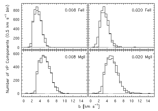
FIG. 4.7 --- The binned distribution of Doppler b parameters from Sim-2. The upper panels are of Fe II and the lower panels are of Mg II. The left panels are of the 0.008 A equivalent width limit and right panels are of the 0.02 A limit. The thick lined histogram is the input distribution. The narrow lined histogram is the distribution resulting from minfit, where the number of clouds has been scaled to match that of the input.
Recovery of the input b distribution is sensitive to the signal to noise. A two-sample Kolomorov-Smirnov (KS) test on the cumulative distributions for the null hypothesis that the measured distributions are consistent with having been drawn from the input distribution yielded probabilities of P_KS =0.956 and 0.003 for the 0.008 A and 0.02 A limit simulations, respectively. That is, the VP decomposition of the 0.02 A limit simulation yielded a minfit b distribution that is not statistically consistent with having been drawn from the input b distribution at the 99.7% confidence level. However, the 0.008 A limit simulation yielded a b distribution that is not inconsistent with having been drawn from the input b distribution. Indeed, the near unity P_KS is suggestive that they are in fact drawn from the same distribution. A KS test that the 0.008 A and 0.02 A limit b distributions are consistent with being drawn from the same underlying distribution yielded P_KS = 0.329. This latter KS test did not yield, to a high confidence level, a result from which the b distributions of the two equivalent width limit simulations could be claimed to be inconsistent with one another.
For both simulations, there is an extended tail below the cutoff, b_min = 3.0 km/s, which is also present in the Fe II b distribution. This artifact of VP parameter minimization techniques was also noted by Lu et al. (1996a). This population of b parameters is not induced by blending effects alone. Not surprisingly, comparison of the 0.008 A limit simulation and the 0.02 A limit simulation did reveal that higher signal to noise in the spectra results in a higher recovery rate of the input b distribution.
4.4.2 Recovering Fe II to Mg II Input Relations
Assessing the degree to which the Mg II and Fe II VP parameters are recovered relative to one another is central to understanding the level at which inferences based upon their comparison are significant. For the following, only the 0.02 A limit simulations are presented, since they serve to illustrate the worse case scenario.
In Figure 4.8, the Fe II VP parameters are plotted verses the Mg II VP parameters output by minfit (the upper panel shows the column densities and the lower shows the Doppler b parameters). In both panels, the dash-dot line gives the locus of Sim-2 input VP parameters, as described for Sim-1C. Down to the Fe II column density completeness, the column densities follow the input correlation with an RMS scatter of ~0.4 dex, but with increased scatter for input columns log N(MgII) > 13.5 cm^-2. This represents the intrinsic (no blending effects) scatter in the relative column densities due to VP decomposition. Since there are five Fe II transitions having a wide range of absorption strengths being simultaneously fit, the Fe II columns output by minfit are well constrained for the full range of input Mg II columns. The increased scatter is predominately due to overestimation of log N(MgII) > 13.5 cm^-2 and underestimation of log N(MgII) < 15.5 cm^-2 input column densities, respectively. It is interesting that the scatter for 14.00 < log N(MgII) < 15.0 cm^-2 input column densities is the least severe over this regime. The intrinsic scatter in the relative column densities due to VP decomposition is a non-monotonic, though increasing, function of the input column density. However, the intrinsic scatter in terms of fitted Mg II columns is a monotonically increasing function, and is roughly 0.4 dex up to log N(MgII) ~ 13.0 cm^-2 increasing to 1.5 dex at log N(MgII) ~ 15.0 cm^-2.
Figure 4.8
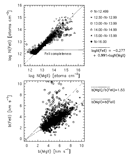
FIG. 4.8 --- The Fe II VP column densities (upper) and Doppler b parameters (lower) plotted against Mg II output by minfit. The dash-dot line gives the locus of Sim-2 input VP parameters (see text). The legend gives the data point types as a function of the input Mg II. The formal error bars are not shown for presentation purposes.
The Doppler b parameters (lower panel Figure 4.8, exhibit a fairly uniform scatter for input log N(MgII) > 12.5 cm^-2 and over all fitted b values. The input relation between the Fe II and Mg II was assumed strictly thermal (as shown by the dash-dot line). Data points either above the 1:1 correlation line (dotted) or below the thermal relation line yield unphysical clouds, if the basis for inferring cloud properties is that the Fe II and Mg II arise in the same clouds having the same internal physical conditions. In the limit that turbulent/bulk motion dominates the line broadening, the Fe II and Mg II b parameters are equal, and fall on the 1:1 correlation line. In the limit that the line broadening is strictly thermal, the Fe II and Mg II b parameters obey the ratio given by Equation 4.7, and fall on the thermal line. The scatter about the thermal (input) relation has an RMS value of ~1 km/s, excluding components with input log N(MgII) < 12.5 cm^-2. The b parameter is less constrained in weak lines than is the column density.
The implications for quantifying the turbulence from VP decompositions of unblended lines seen in HIRES spectra with signal to noise ratio of roughly 30, are that (1) lines with fitted column densities log N(MgII) > 13.0 cm^-2 should be used, and (2) the uncertainty due to the intrinsic scatter from the VP fitting should be fairly constant as a function of fitted b(MgII). It is cautioned that the former selection criterion may introduce a bias in that larger column components may arise in the regions of clouds undergoing physically distinct dynamics as compared to those arising in regions giving rise to the smaller column densities.
4.4.3 Inferred Turbulence in Thermal Clouds
A fundamental measurement is the contribution of a turbulent component in the absorption line broadening, which can be obtained from the simplified relation,

It is assumed that the turbulent or bulk motion is a Gaussian contribution to the isothermal line broadening (both unlikely physical scenarios in the real world). This technique has recently been applied to C IV at z ~ 2.5 by Rauch et al. (1996). Solving for b_turb yields the relation

where r = m(Mg)/m(Fe) = 0.654, and b(MgII) and b(FeII) are the measured VP parameters output by minfit. Similarly, solving for the thermal b of Mg II yields

For the following, only the 0.02 A limit simulations are presented, since they serve to illustrate the worse case scenario.
In Figure 4.9, results of the deconvolution of the Mg II Doppler b parameter output by minfit are illustrated. The inferred turbulent and thermal component of Mg II clouds are plotted versus the total b(MgII). Only components for which the inferred cloud properties were physical have been included in the deconvolution. Furthermore, only components with fractional uncertainties in their b parameters less than 20% were included. These particular selection criteria resulted in 331 components. Additionally, these criteria culled out all clouds with log N(MgII) < 12.5 cm^-2, as expected (see Figure 4.8) by the large intrinsic scatter in the b parameters for these components.
Figure 4.9
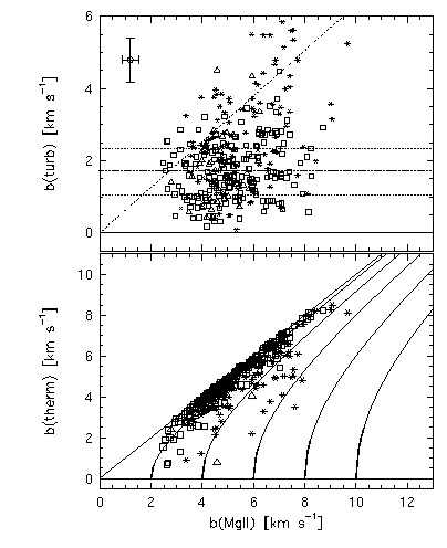
FIG. 4.9 --- The inferred turbulent (upper) and thermal (lower) component of Mg II Doppler b parameter. The dash-dot line gives the locus of values beyond which the turbulent component dominates the line broadening. The horizontal dotted lines give the mean turbulent component and its standard deviation. The average errors are given in the upper left corner. In the lower panel the solid curves are lines of constant turbulent motion.
The intrinsic inferred turbulence for these purely thermal clouds, based upon VP decomposition of signal-to-noise ~ 30 HIRES spectra, can be deduced two ways. The first approach is to compute the mean turbulence from the means of the measured b and the inferred thermal b,

where the means are mean b(MgII) = 5.34 +/- 1.11 km/s and b^2_therm(MgII) = 4.75 +/- 1.14 km/s. The second approach is to measure b_turb directly from the data, which is 2.07 +/- 0.89 km/s. This former approach yields a value statistically consistent with a null non-thermal component, whereas the latter yields a 2-sigma non-thermal component. The mean thermal b parameter of 4.74 km/s yields an inferred mean temperature of 32,000 K, which is comparable to the mean input temperature of 34,000 K. The above quoted values are influenced by the relatively larger scatter in the 12.5 < log N(MgII) < 13.0 cm^-2 components (appear as stellated points in Figure 4.9). As suggested above, if these components are removed from the sample, leaving 228 data points, then the mean turbulence broadening measured directly from the data is 1.71 +/- 0.65 km/s. The effects on the mean thermal broadening are negligible, yielding 4.72 +/- 1.11 km/s. Thus, it appears that including components with column densities in the range 12.5 < log N(MgII) < 13.0 cm^-2 does not introduce a significant bias in the inferred value of the cloud temperatures.
4.5 SIMULATION 3: EFFECTS FROM BLENDING
The simulations designed to access blending required trial input distributions be investigated so that the simulated profiles could be compared to the observed profiles and a satisfactory "match" could be obtained. Since, in real absorbing systems, the velocity clustering and number of "clouds" varies from system to system, it is difficult to motivate quantitative tests to compare the synthetic and observed profiles. Such tests are not likely to yield a definitive, and certainly not unique, set of assumed input parameters. Lu et al. (1996a) performed both an intensity distribution and a power spectrum test to quantitatively "screen" trial simulations of the Ly-alpha forest for selecting their assumed input distributions. For the metal systems, a single distribution function (DF) of the form

where the distribution of the number of clouds per system is,

the distribution of column densities above N_min is,

the distribution of Doppler b parameters above b_i,min is,

and the distribution of velocities is,

has a daunting number of free parameters. Here, the multiple Gaussians are included because the best preliminary fits for observed systems (in that they were performed on binned data) of the Doppler b and velocity distribution were double Gaussians. The second Gaussian was needed to account for an extended tail in each distribution. However, one point of these simulations to ascertain if the extended tail is really present in the observed systems or if it is an artifact of VP component blending. On the other hand, the multiple Gaussians may in fact account for the possibility that the absorbing systems are comprised of more than one population of systems.
In practice, exploring such a large parameter space using "quantitative" minimization schemes is somewhat impractical. A more direct approach is to obtain the DF parameters directly from fitting the observed systems. In fact, this process led to the functional form of the DF, Equation 4.13. However, this technique yielded synthetic profiles that were qualitatively dissimilar to the observed ones! This implies that either the systems are not well described, as a single population, by Equation 4.13, or that the large aforementioned tails in the b and velocity distributions are artifacts of the VP decomposition.
Ultimately, measuring the effects on VP parameters due to component blending in an ensemble of spectra does not require that the synthesized systems are drawn from an input DF that, once analyzed, yields the same DF parameters as obtained for the observed systems. The upshot is that the basic effects of blending can be determined, though they may be a limiting case depending upon the chosen parameters for the distribution function, Equation 4.13.
After visual examination of trial simulations that included Gaussian b distributions, number of cloud distributions, and kinematic velocity distributions, a final set of input distributions was selected: (1) The column density power law distribution was chosen to have slope delta = 1.57, based upon preliminary fitting to the observed systems and consistent with that used for the single component simulations. The column density cutoffs were log N_min(MgII) = 11.5 and log N_max(MgII) = 15.5 cm^-2. The former is the completeness limit of unblended lines for the 0.008 A limit simulation. (2) The number of clouds was set to 10 for all systems. By holding the number of clouds at a constant per system, the simulation can be used to infer the level at which information is lost and blurred. (3) The b parameter distribution was drawn directly from those obtained by VP fitting the observed systems with minfit. The single narrow Gaussian used for the single component simulations yield too few systems with broad saturated profile morphology. (4) A single Gaussian kinematic spread of cloud velocities was assumed for all systems. The observed systems, when the clouds velocities are binned with Delv = 10 km/s, are best fit by a double Gaussian. However, a double Gaussian DF did not yield simulated profiles qualitatively similar to those in the HIRES spectra. The narrower of the two Gaussian spreads, sigma = 45.2 km/s, was used. That the double Gaussian velocity spread did not reproduce profiles that qualitatively match even a small fraction of the observed profiles may imply that the kinematics of Mg II systems are not comprised of a single population. (5) The five Fe II transitions, listed in Table 2.1, were fit simultaneously using the same Fe II to Mg II column density and Doppler b relations as was done for Sim-1C. The clouds were assumed to be broadened strictly by thermal internal motions. (6) In order to examine the effects due to the signal to noise ratio, two simulations were carried out. The limiting equivalent widths were 0.008 A and 0.02 A.
In Figure 4.10 and Figure 4.11, 100 simulated Mg II 2796 transition and the VP decomposition models are presented. Though the full VP model was obtained by simultaneously fitting the Mg II 2796, 2803 doublet and five Fe II transitions, only the 2796 transition is shown for this grid. In Figure 4.10, 50 simulations using the 0.008 A limiting equivalent width are shown. In Figure 4.11, the same 50 systems are shown but with a 0.02 A equivalent width detection threshold. Immediately, one can compare the number of VP components found for both simulations, and examine under what conditions they are different. In Figure 4.12, the full compliment of fitted transitions and the VP models for System #071 is illustrated for the 0.02 A limit simulation.
Figure 4.10
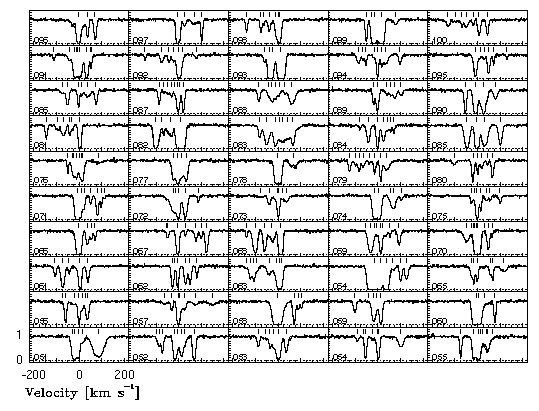
FIG. 4.10 --- A grid of the Mg II 2796 transition and the minfit model for blending simulations 50-100 with limiting equivalent width 0.008 A.
Figure 4.11
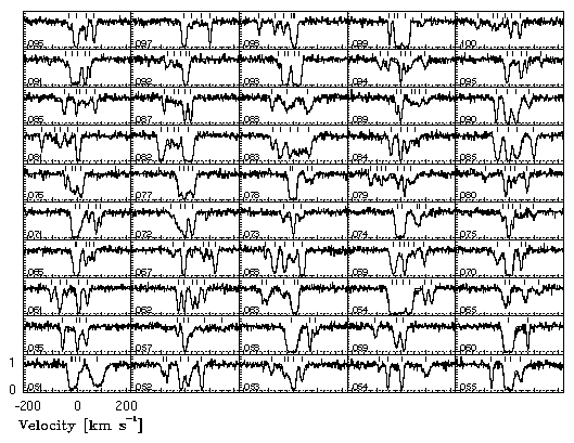
FIG. 4.11 --- A grid of the Mg II 2796 transition and the minfit model for blending simulations 50-100 with limiting equivalent width 0.020 A.
Figure 4.12
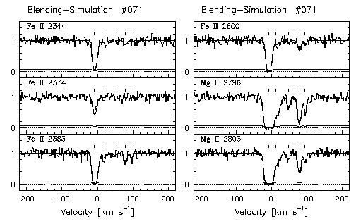
FIG. 4.12 --- Blending Simulation #71 for the 0.02 A limit simulation, showing the (partial) compliment of Fe II transitions simultaneously fit by minfit.
The fitting process involved running the modified version of autovp on the Mg II 2796 transition. The autovp Mg II VP parameters were then scaled for the Fe II transitions using Equation 4.6 and Equation 4.7. The VP parameters where then handed to minfit and the full VP model was chi^2 minimized. This technique worked roughly 95% of the time. For the other 5%, usually systems with broad saturated Mg II profiles, the autovp model (including the Fe II parameters) was edited by hand using profit before minimization with minfit.
4.5.1 Effects on the Number of Components per System
In the left hand panels of Figure 4.13, the binned distribution of the number of clouds per system are shown for both the 0.008 A and 0.02 A limit simulations. The vertical dotted line is the input number of components per system. For an ensemble of systems all having the same number of input components, these distributions reveal that the spread in the number of fitted components increases with increasing signal to noise. Furthermore, it can be seen that the mean number of components approaches the input number as signal to noise is increased.
4.5.2 Effects on the Inferred Distribution of Column Densities
The right hand panels of Figure 4.13 show the binned distribution of column densities for both the 0.008 A and 0.02 A limit simulations. The solid curve is the input distribution of column densities, given by Figure 4.15. The shaded region gives the range of column density "partial completeness". Here, the term partial completeness, for a single equivalent width system, is defined such that the lower limit is the total completeness of unblended components and the upper limit is total completeness for blended components. The term takes on a different meaning when the sample of systems are comprised of a range of equivalent width limits. In such cases (as with Sample B), partial completeness is defined such that the lower limit is the total completeness of the unblended components in the lowest equivalent width threshold spectrum of that sample, and the upper limit is total completeness for the blended components in the highest equivalent width threshold spectrum of that sample.
Figure 4.13
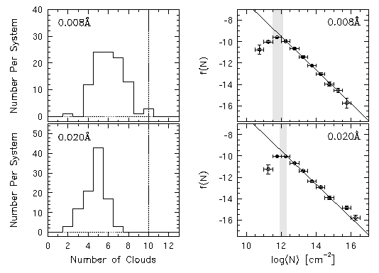
FIG. 4.13 --- The number of clouds per system and the distribution of Mg II column densities. Top panels are from the 0.008 A spectra and lower panels are the 0.020 A spectra. The shaded regions give the range over which partial completeness is occuring (see text).
The upper boundary to the column density completeness was determined by simply varying N_min, and obtaining the maximum likelihood value of the power-law exponent in Equation 4.15 (see Section 5.1.1). The results are given in Table 4.1. The value of N_min which yields a delta consistent with the input value, delta = 1.57, is the column density above which "all" column densities are detectable when blending is causing incompleteness above the detection limit (non-blended components).
Table 4.1
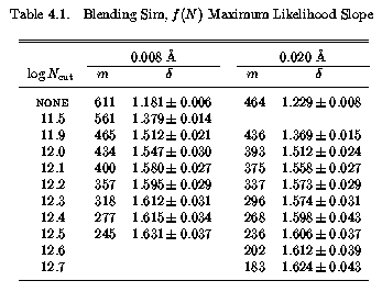
The deduced range of partial completeness for the 0.008 A limit simulation is approximately 11.5 < log N_cut(MgII) < 12.1 and for the 0.008 A limit simulation is approximately 11.9 < log N_cut(MgII) < 12.3. Apparently, the upper limit for the 0.02 A limit simulation is not as well determined as for the 0.008 A limit simulation, implying that the completeness limit due to blending becomes more "blurred" as the signal to noise is decreased. It is also apparent from Figure 4.13 that the the column density completeness limit for unblended components (lower limit of shaded regions) is more sensitive to the spectral signal to noise than is the completeness limit for blended lines. This can be seen by the fact that the region of partial completeness has become narrower for the 0.02 A limit simulation, which occurred because the lower limit of the shaded region migrated to larger columns more rapidly than the upper limit. One might surmise that the region of partial completeness would converge as the signal to noise is further decreased, meaning that the unblended and blended component detection thresholds would be one in the same.
It is important to point out that if one ignored the region of partial incompleteness, and naively used the maximum likelihood method using the N_min for the non-blended components, then the inferred column density distribution power would be underestimated (too shallow). Either one needs to apply a correction factor to elevate the number of column densities in this regime, or one needs to limit the maximum likelihood technique to those column densities for which there is total completeness. A similar conclusion was reached by Lu et al. (1996a) and by Hu et al. (1995) for the Ly-alpha forest.
4.5.3 Recovering the Fe II to Mg II Input Relations
In Figure 4.14, Fe II and Mg II column density and Doppler b VP parameters and their errors output by minfit are plotted against one another. The sample shown has been selected using the criteria discussed in Section 4.1.1. For the upper panels, the data points shown include the full range of column densities (the completeness cutoff has not been applied), for illustration purposes. The shaded regions illustrate the range of partial completeness for the respective equivalent with limits. The dot-dash line is the input relation for the Fe II and Mg II column densities, given by Equation 4.6.
Figure 4.14
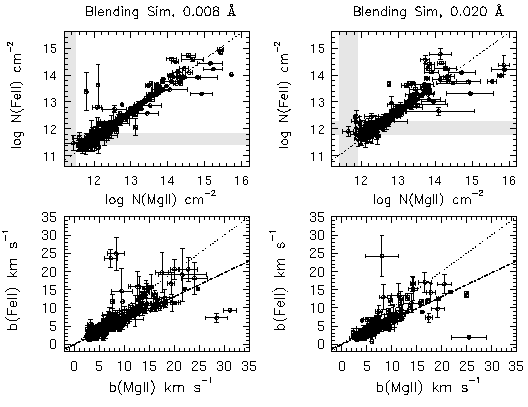
FIG. 4.14 --- Fe II verses Mg II VP parameters output by minfit for the Blending Simulations. The left panels are from the 0.008 A limiting equivalent width spectra and the right panels are from the 0.020 A spectra. The shaded grey areas show the region where the completeness for unblended VP components falls from full to null detections.
Formal fits to the data, assuming the relation

yield a = 0.985 +/- 0.004 and b = -0.184 +/- 0.042 for the 0.02 A limit simulation and a = 1.006 +/- 0.012 and b = -0.433 +/- 0.141 for the 0.008 A limit simulation. The fit incorporated the uncertainties on both the Fe II and the Mg II column densities (Press et al. 1986), and included column densities only in the regime of total completeness. Both simulation results are comparable to the input values a=0.991 and b=-0.277. For both simulations, the scatter of the data about the fitted correlation line is larger than the formal uncertainties in the column densities, as can be measured by the fit reduced chi^2 = Var(fit)/[nu x Var(data)], where nu is the degrees of freedom. The scatter appears to not increase rapidly with signal to noise; for the 0.02 A limit simulations chi^2 = 10.1 and for the 0.008 A limit simulations chi^2 = 8.7. Since the simulation equivalent width limits are the same as for the observed Sample B, it would seem reasonable to assume that if the scatter in the observed N(FeII) to N(MgII) fitted relation yields a chi^2 significantly larger 10, then the scatter represent real variations in column ratio from absorbing system to absorbing system. This is especially likely to be true in the regime log N (MgII) < 14.0, where the scatter due to the VP decomposition is much smaller in comparison to the higher Mg II column densities that dominate the value of chi^2.
In the lower panels of Figure 4.14, the Doppler b parameters are plotted. The sample selection was described in Section 4.1.1. The thermal relation (Equation 4.7) is given by the dot-dash line and the 1:1 correlation line is given by the dotted line. Doppler b parameters that lie outside these curves yield unphysical inferred cloud properties. The best measure for how well the b parameters have been recovered is the inferred cloud properties, especially any non-turbulent motion "contribution" to the line broadening.
4.5.4 Inferred Cloud Thermal/Non-Thermal Properties
In Figure 4.15, the inferred turbulent component (Equation 4.10, upper panels) and the thermal component (Equation 4.11, lower panels) verses the measured Mg II Doppler b parameter are shown for both equivalent width simulations. The sample selection was more stringent than that described in Section 4.1.1, in that the fractional errors in the total b parameters were chosen to be smaller than 20%. Additionally, only components that yielded physical cloud properties were selected. These added selection criteria resulted in 103 components for the 0.008 A limit simulation, and 50 components for the 0.02 A limit simulation. For the upper panels (turbulent b), the dash-dot line separates the regime at which the turbulent component dominates the line broadening. For reference, the horizontal dotted lines give the mean turbulent component for the unblended lines analyzed from Sim-2 (see Figure 4.9). For the lower panels (thermal b), the solid curves are lines of constant turbulent motion.
Figure 4.15
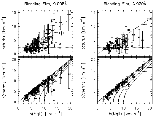
FIG. 4.15 --- The inferred turbulent (upper panels) and thermal (lower panels) contributions to the total Doppler b parameters. Left hand panels are from the 0.008 A spectra and right hand panels are the 0.020 A spectra.
For both blending simulations, there is a clear correlation between b_turb and b(MgII) that would result in a systematic underestimation of the cloud temperatures with increasing b(MgII). Overall, the cloud properties are inferred to be quiescent, or thermally dominant. It appears that blending does not significantly elevate the inferred turbulent component over that which was inferred from the simulations of the unblended components. As such, the predominate effect giving rise to an inferred non-thermal component, when the clouds are known to be purely thermal, is the noise in the spectra and not the clustering properties of the components. The apparently smaller scatter in the 0.02 A limit simulation is an artifact of the sample selection criteria, and is not real.
4.5.5 Effects on the Doppler b and Velocity Distributions
In Figure 4.16, the binned distributions of the Mg II Doppler b parameters (upper left panel) and of the cloud velocities (upper right panel) are shown. The thick solid histogram is the input distribution, whereas the thin solid line is the 0.008 A limit simulation and the dotted line is the 0.02 A limit simulation. In the lower panels, the respective cumulative distributions functions (CDFs) are shown. These distributions are useful for two important reasons. First, direct comparison of the VP decomposition CDF to the input CDF immediately reveals the ranges where under populations and/or over populations are present in the distribution. Second, using a Kolomorov-Smirnov test, the the CDFs can be directly compared to test the null hypothesis that they are statistically consistent with having been drawn from the same underlying distribution.
Figure 4.16
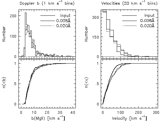
FIG. 4.16 --- The Doppler b distribution for the Mg II clouds and their velocity distribution. The curves have been normalized to the number of input pairs. Top panels are the binned distributions and lower panels are the normalized cumulative distribution functions.
For the following analysis, the sample used for the discussions involving b parameters is that following application of the selection criteria. However, the full sample has been used for discussions involving the velocity distributions.
4.5.5.1 Doppler b Distributions
There is a tendency for narrow b parameters, which are not present in the input, too appear in the range b<3 km/s. These are likely due to narrow components that, for example, are placed in an asymmetric wing of a broader profile. Similar results have been have been found by Lu et al. (1996a) and Rauch et al. (1992, 1993).
A two-sample KS test of the null hypothesis that the measured distributions are consistent with having been drawn from the input distribution yielded probabilities of P_KS = 0.021 and 0.005 for the 0.008 A and 0.02 A limit simulations, respectively. That is, the VP decomposition of the low signal to noise simulation yielded a minfit b distribution that is not consistent with having been drawn from the input distribution, whereas the high signal to noise simulation yielded a b distribution that is. A two-sample KS test that the 0.008 A and 0.02 A limit b distribution are consistent with being drawn from the same underlying distribution yielded P_KS = 0.155. Interestingly, the output b distributions from the two equivalent width limited simulations are not inconsistent with being drawn from the same distributions. This is surprising in view of the fact that they are not both consistent with the input distribution, which is apparent in the broadening of the distribution with increasing limiting equivalent width in Figure 4.16. As with the single component simulations, the distribution of Doppler b parameters obtained by a VP decomposition is sensitive to the signal to noise in the spectra. The somewhat disturbing consequence of this result is that measured b distributions are a function of both the signal to noise in the spectra and the severity of the component blending.
4.5.5.2 Velocity Distributions
A two-sample KS test of the null hypothesis that the measured distributions are consistent with having been drawn from the input distribution yielded probabilities of P_KS ~ 4 x 10^-6 and ~ 5 x 10^-5 for the 0.008 A and 0.02 A limit simulations, respectively. That is, the VP decomposition of both simulations yielded minfit velocity distributions that are not statistically consistent with having been drawn from the input velocity distribution. There is a distinctive broadening of the velocity distributions, as seen in the binned data (upper panel of Figure 4.16). Visual inspection of the velocity CDFs reveals that the VP decomposition results are more closely matched to one another than to the input distribution over all observed velocities. A two-sample KS test that the 0.008 A and 0.02 A limit velocity distributions are consistent with being drawn from the same underlying distribution yielded P_KS = 0.73. Since only a single input kinematic distribution has been examined, nothing quantitative can be said about sensitivity to the underlying kinematics. However, it would seem likely that the inferred distribution would indeed be sensitive.
The broadening in the velocity distribution can be quantified by fitting a Gaussian to the binned data. The input distribution is measured to have sigma = 45 km/s, which is consistent with the simulation input value. However, the resulting velocity dispersion for the 0.008 A limit simulation is sigma = 61 km/s and for the 0.02 A limit simulation is sigma = 64 km/s.
Examining the log N(MgII) - b plane is useful because it allows a visualization of the populations of clouds and their distributions that result from VP decomposition of absorption profiles. Furthermore, comparing the input to the resulting output, both before and after the sample selection criteria are applied, may lead to additional insights on portions of the plane that are affected by the VP decomposition approach.
In Figure 4.17, the log N(MgII) - b plane is shown for the input VP parameters, for all the resulting cloud VP parameters from minfit, and for the sample resulting from the selection criteria outlined in Section 4.1.1. The 0.008 A limit simulation is presented in the center two panels and the 0.02 A limit simulation is presented in the right two panels. The input distribution is shown in the lower left-most panel. Recall that the input distribution of Doppler b parameters was drawn from the distribution obtained by VP decomposing the HIRES data, whereas the column density distribution was taken from a single power law. This explains two features in the log N-b plane for the input parameters: (1) the same b parameter could in principle be drawn from the observed distribution more than once, and thus there is some clustering of the Doppler parameters, and (2) the power law fall off of large column densities and the low number of large-b parameters resulted in no large-N large-b clouds. Thus, this portion of the plane has not been sampled with these simulations. It is interesting to note that Lu et al. (1996a) did sample this portion of the plane and suggested that a lack of measured large-N large-b clouds was an artifact of VP decomposing absorption profiles. It may be that these clouds are present in nature, but that the fitting to the HIRES data has not recovered them.
Figure 4.17
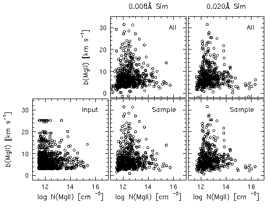
FIG. 4.17 --- (lower left panel) The input distribution shown in the log N-b plane. -- (upper panels) All resulting VP components for the 0.008 A limit simulation (left) and the 0.02 A limit simulation (right). -- (lower panels) The same, after the sample selection criteria have been applied (see text).
The types of clouds resulting from the VP decomposition and the effects of both signal to noise and the sample selection criteria can be inferred by studying Figure 4.17. Large-N small-b clouds appear to result from lower signal to noise in the spectra, as can be seen by the population of points with log N(MgII) > 15.5 cm^-2 in the 0.02 A limit simulation. These clouds are not present in either the input nor the 0.008 A limit simulation. Further, these clouds have small fractional errors, since they survived the process of sample selection.
Another artifact of the fitting process that is also signal to noise dependent appears to be the non-recovery of small-N large-b clouds. There is a deficit of clouds with b > 10 km/s for column densities near the detection thresholds in both simulations. Note that this leads to a bias towards small-N small-b clouds, which is easily understood in terms of higher continuum depression in the case of smaller b parameters. It is not unlikely that this bias could result in an "induced" correlation between b parameters and columns densities.
Spearman-Kendall rank correlation tests were used to investigate if a significant correlation had been induced by this biasing effect. The Spearman-Kendall results are presented in Table 4.2 and Table 4.3. For both the 0.008 A limit and 0.02 A limit simulations, the tests reveal that the input parameters are consistent with the null hypothesis of no correlation. In fact, the tests yielded negative correlation coefficients, indicative of an anti-correlation trend between the input parameters. For the total sample (labeled "All"), the tests reveal that the relationship between the 0.008 A limit simulation VP column densities and b parameters are consistent with no correlation with very small probability, P = 0.0007. In other words, no correlation can be ruled out at the 99.9% confidence level (this is technically distinct from claiming a correlation to some confidence level, since the Spearman-Kendall tests do not measure this). Such a high level of confidence does not result for the 0.02 A limit simulation. It appears that blending in high signal to noise spectra may indeed induce a correlation between the column densities and b parameters. Once the selection process is used to cull out VP parameters with relatively large fractional errors, the tests reveal that the correlation in the 0.008 A limit simulation (labeled "Sample") remains suggestive, since a 97% confidence level (2.1-sigma result) is found that the data are inconsistent with no correlation. No such trend in the Spearman and Kendall probabilities is seen for the 0.02 A limit simulation tests.
Table 4.2
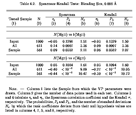
Table 4.3
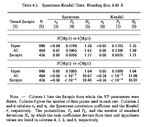
Though the statistics are not overwhelming, the above analysis is suggestive that the higher the signal to noise in the spectra, the more likely is an apparent correlation in the log N - b plane. It is interesting to note that the 0.02 A limit simulation may not show the putative induced correlation because of the abundance of large-N small-b clouds. On the other hand, it is possible that had the large-N large-b quadrant of the log N - b plane been sampled by the input parameters, the statistics suggestive of an induced correlation may have been more compelling.
The line of sight velocity clustering properties of the absorbing clouds is one of the many important clues useful for understanding the overall nature of absorbing gas. It is important to keep in mind that, in practice, the velocity zero point of any absorption profile is set arbitrarily. This shall remain the case for most observed systems until the redshifts of the galaxies associated with the absorbing gas have been measured to a high accuracy (i.e. < 30 km/s). More generally, as was done above, the clustering properties are measured in relative terms. Since the velocity zero point has been set at the optical depth median (see Section 2.2.3), the largest column density clouds are likely to have small velocities. But there is no a priori reason (that is, without invoking a kinematic model) to assume that these large-N clouds are not found with somewhat equal frequency over the full range of measure velocities. A correlation, anti-correlation, or lack of correlation in the v-log N plane may in fact provide strong support for a given model of cloud kinematics. Based upon the predicted cloud velocity distributions of Lanzetta & Bowen (1992), for example, a single population of their radial infall models would not be expected to result in a strong correlation or anti-correlation, but would likely result in a flat distribution of column densities with velocity. On the other hand, a single population of their rotation or disk-like kinematic models would be expected to yield a fairly clear anti-correlation in the v - log N plane.
In Figure 4.18, the v - log N(MgII) plane is shown for the input VP parameters, for all the resulting cloud VP parameters from minfit, and for the sample resulting from the selection criteria outlined in Section 4.1.1. The 0.008 A limit simulation is presented in the center two panels and the 0.02 A limit simulation is presented in the right two panels. The input distribution is shown in the lower left-most panel.
Figure 4.18 is interesting to examine because its study can provide insights to possible biasing in the population of clouds recovered from the VP decomposition. According to the Spearman-Kendall tests, the input column densities and velocities are not correlated. Yet, for both the 0.008 A limit and 0.02 A limit simulations, the probabilities that the column densities are not correlated with the velocities are vanishingly small.
Figure 4.18
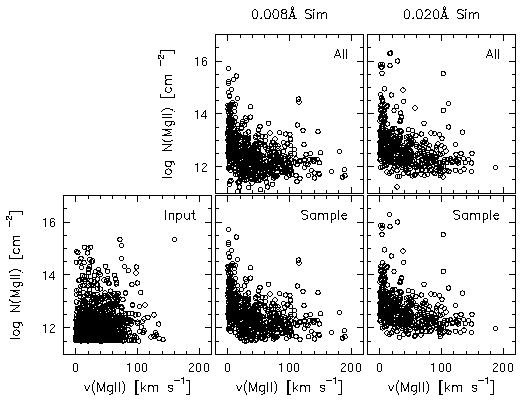
FIG. 4.18 --- (lower left panel) The input distribution shown in the v-logN. -- (upper panels) All resulting VP components for the 0.008 A limit simulation (left) and the 0.02 A limit simulation (right). -- (lower panels) The same, after the sample selection criteria have been applied (see text).
There are two effects that contribute to this induced correlation: (1) the zero point of the velocities for the output data have been shifted so that large columns preferentially have small velocities, and (2) small-N clouds have not been recovered (on average four clouds are not recovered for the 0.008 A limit and six clouds are not recovered for the 0.02 A), particularly in the regions where large-N clouds are blended. This 40-60% of the cloud population that has been "blanketed" by large-N clouds would have populated the log N < 12.3 cm^-2 and v < 40 km/s area in the v - log N plane. It is because of the velocity shifting that these clouds are preferentially lost at small velocities. Had the input data been drawn from, for example, the infall model of Lanzetta & Bowen (1992), so that large-N clouds preferentially had v ~100 km/s, then the effect may have been quite different. However, since nonsymmetric horned profiles could still result in the velocity zero point that gave the impression seen in Figure 4.18, it is not clear how the stochastic inherent in small number statistics would affect the resulting distribution on the v - log N plane.
The bottom line is that any anti-correlation inferred from the VP decomposition of HIRES data may in fact be due to the blanketing of small-N clouds in the regions of the deep and broad regions of the absorption profiles, which are preferentially at small velocities. This precise effect could be giving rise to the broadening in the cloud velocity distribution.