We have encountered the concept of least-squares fitting several times: once to derive extinction and transformation coefficients and zero points, and again when we talked about crowded field photometry. Least squares fitting has a very large number of applications in science in general, as it is a commonly used technique to determine the parameters of some model which one wishes to fit to their data.
The concept of least-squares fitting has a statistical basis when one
considers a set of observations which arise from a system which can
be described by some mathematical model but where the observations have
errors which are normally distributed around the predicted model values.
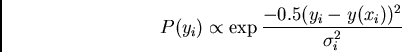
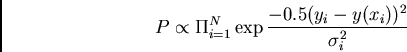
In this case, we can write the probability of observing any particular
data point given a model, ![]() :
:
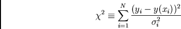
This is the standard least-squares equation: one wishes to minimize the
sum of the square of the differences between observation and model by
adjusting the model parameters. We define this quantity as ``chi-squared'',
or ![]() . For a good fit, one would expect that on average, points
deviate from the model by roughly
. For a good fit, one would expect that on average, points
deviate from the model by roughly ![]() , so one would expect a
, so one would expect a
![]() for a set of
for a set of ![]() observations to approach
observations to approach ![]() if the model is
a good model and the errors have been estimated properly. In fact, it
is possible given an observed value of
if the model is
a good model and the errors have been estimated properly. In fact, it
is possible given an observed value of ![]() to compute the probability
that this value would be obtained if the model is correct; this allows
one to judge the quality or likelihood that the model which minimizes
to compute the probability
that this value would be obtained if the model is correct; this allows
one to judge the quality or likelihood that the model which minimizes
![]() is actually the correct model. One often discussed the
reduced
is actually the correct model. One often discussed the
reduced ![]() quantity,
quantity, ![]() , which is just
, which is just ![]() divided
by
divided
by ![]() , where
, where ![]() is the total number of points, and
is the total number of points, and ![]() is the number
of free parameters in the fits; the latter is there because any set
of observations which does not have more data points than the number of
free parameters can generally be fit perfectly even for an incorrect
model. The total
is the number
of free parameters in the fits; the latter is there because any set
of observations which does not have more data points than the number of
free parameters can generally be fit perfectly even for an incorrect
model. The total ![]() is called the degrees-of-freedom of the fit.
is called the degrees-of-freedom of the fit.
How does one do least-squares in practice? Basically, one wishes to
minimize ![]() with respect to one or more parameters of a model.
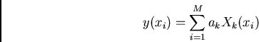
Let us first consider models which can be written in the form:
with respect to one or more parameters of a model.
Let us first consider models which can be written in the form:
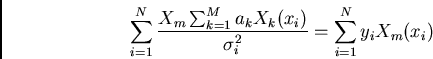
![\begin{displaymath}\chi^2 = \sum_{i=1}^N \left[ y_i - \sum_{k=1}^M a_k X_k(x_i)\over \sigma_i\right] ^2\end{displaymath}](img597.png)
![\begin{displaymath}\sum_{i=1}^N 2 \left[ y_i - \sum_{k=1}^M a_k X_k(x_i)\over \sigma_i\right] (-X_m(x_i)) = 0\end{displaymath}](img599.png)
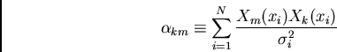
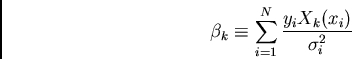
If we define a matrix, ![]() , to be
, to be
Associated with solving for the ``best'' parameters, one often wishes to
compute the errors associated with the fit parameters. This is discussed
in Numerical Recipes (chapter 15), with the result:
One can also consider the situation where a model is non-linear in
the parameters, ![]() , i.e., the derivatives with respect to each parameter
may depend on the parameter value. This leads to non-linear least squares
techniques. These are more complex, as one can have situations where there
are many minima in
, i.e., the derivatives with respect to each parameter
may depend on the parameter value. This leads to non-linear least squares
techniques. These are more complex, as one can have situations where there
are many minima in ![]() and one needs to find the global minimum rather
than a local one. Such problems require a starting guess of a reasonable
solution and then iteration towards the best solution. The crowded field
photometry problem falls into this category because the model is nonlinear
in the position parameters.
and one needs to find the global minimum rather
than a local one. Such problems require a starting guess of a reasonable
solution and then iteration towards the best solution. The crowded field
photometry problem falls into this category because the model is nonlinear
in the position parameters.