3. THE ABSORBING SYSTEMS
The analysis of the Mg II systems in the HIRES spectra, based upon the discussion of the previous chapter, is presented. The analysis of each system includes measurements of the equivalent widths (or detection limits), doublet ratios, velocity widths, velocity asymmetries, profile shapes, the integrated apparent column densities, and the number of subfeatures. For each subfeature, the equivalent widths (or detection limits), doublet ratios, velocity widths, velocity asymmetries, profile shapes, and the integrated apparent column densities are also measured. In addition, each subfeature velocity centroid is measured. Formal uncertainties in all quantities are computed. In addition to these direct measurements of the absorption spectra, a full VP decomposition of each system is presented. There are some cases where a VP decomposition is not well suited, such as when the profiles are very saturated and additional information is not available from the Fe II or Mg I transitions. Each absorption system is individually discussed in Section 3.3.
3.1 ABSORPTION PROPERTIES OF THE OBSERVED SYSTEMS
The overall Mg II profile and absorption properties are presented in Table 3.1 and Table 3.2. Table 3.1 lists (1) the absorber redshift, (2) the uncertainty in the redshift in velocity units, sigma(v) [km/s], (3) the velocity width, omega(v), velocity asymmetry, eta(v), and rest-frame equivalent width, EW(rest), of the 2796 transition, and (4) the Mg II doublet ratio, DR. Not tabulated is a quantity that will be referred to as the profile "shape parameter", eta(v)/omega(v). This parameter essentially measures the velocity width normalized asymmetry and is more useful for characterizing profile shapes because the asymmetry is simply a higher moment of the velocity width. Thus, a "wide" line with a given profile morphology will necessarily have a larger eta(v) than will a "narrow" line with the identical morphology. A null shape parameter denotes perfect symmetry about the profile velocity zero point. A negative shape denotes extended blue wings and a positive shape denotes extended red wings.
Table 3.1
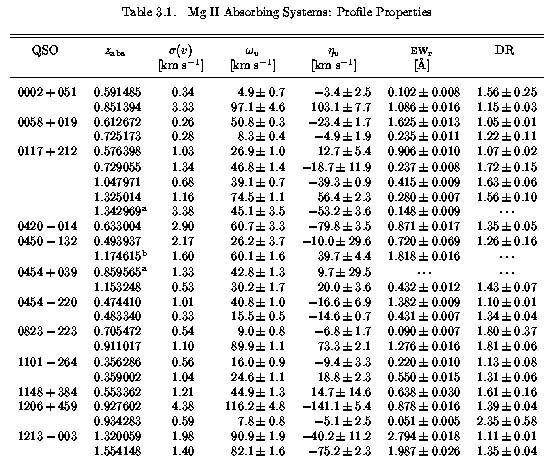
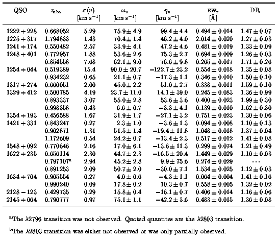
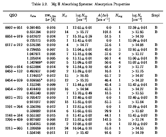
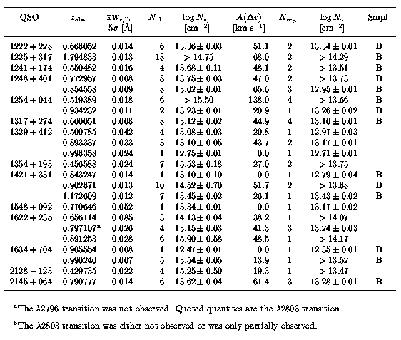
Table 3.2 lists the 5-sigma EW(rest) detection limit for the Mg II 2796 profile for each system. Also listed are (1) the number of VP components, (2) the integrated VP column density of Mg II 2796, and (3) the "absolute deviation from the median" of the cloud velocities, given by

where Dv(i) = v(i)-v, and v is the median cloud velocity. The median is used in lieu of the average because the former is symmetric about the number of clouds and is not sensitive to one or a few large Dv(i) clouds. Also tabulated, are the apparent column densities, measured directly from the Mg II 2796 profiles, and the number of "kinematic subsystems", or profile subfeatures. The last column provides the sample designation for the system (see below).
Table 3.2
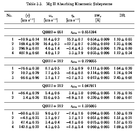
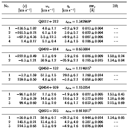
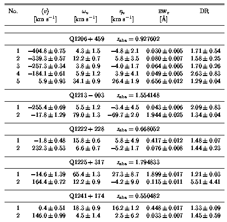
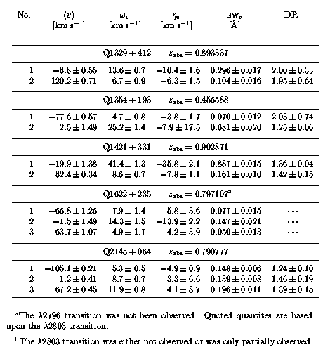
The number of "kinematic subsystems", and each subfeature velocity centroid, v, velocity width, Mg II 2796 EW(rest), and Mg II DR are given in Table 3.3. In Table 3.6 through Table 3.54, the absorption properties of each system are presented. Each table lists the adopted integrated apparent column density for Mg II, Fe II, Mg I, Mn II, and Ca II for the kinematic subsystems and for the overall system. If there is a null feature detection for a given ion, then upper limits are given. In the case of unresolved saturation, the lower limit is quoted. Also listed are the rest-frame equivalent widths, EW(rest), of the transitions listed in Table 2.1. In the case of null detections, the upper limit of EW(rest) is quoted.
Table 3.3

The HIRES spectra of all identified ion transitions given in Table 2.1 are presented for each absorbing system in Figure 3.15 through Figure 3.62. The minfit VP decomposition model spectra are also shown superimposed over the data, where the ticks above the continua give the velocity centroid of each VP component. Recall that all transitions within a system were fit with the same number of components, so that often Fe II, Mg I, or Ca II show no discernible absorption where a VP component has been found based upon Mg II. The column densities of these components were always consistent with zero, and have not been included in the analysis. In Table 3.55 through Table 3.81. the VP velocity centroids, column densities, and Doppler b parameters are given. In the case where the column density is consistent with zero, no entry is given.
Since a deeper appreciation of the uncertainties inherent in the VP decomposition technique was sought, a fairly comprehensive set of simulations were performed. These simulations and the subsequent analysis of the VP decomposition of the simulated spectra are presented in Chapter 4. The limiting detectable column density for Mg II is presented in Figure 4.2. Analysis of the VP components obtained for the HIRES spectra is given in Chapter 5.
3.2 REDSHIFT DISTRIBUTION AND DETECTION SENSITIVITY
The redshift distribution of the Mg II systems is illustrated in Figure 3.1. Two samples have been defined based upon the EW(rest) detection threshold. Sample A includes all 48 systems. Sample B includes only those systems for which the 5-sigma EW(rest) detection limit of the Mg II 2796 transition is less than 0.02 A. Sample B is shown as the shaded histogram. As illustrated in Figure 3.2, there is a natural break in the EW(rest) distribution at 0.02 A, below which 37 of the 48 systems are found. There are two additional reasons this EW(rest) limit was chosen.
Figure 3.1
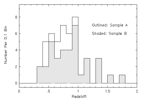
FIG. 3.1 --- The number of observed systems per 0.1 redshift bin. The thick line histogram shows the full sample presented in Table 3.1, and the shaded region gives the distribution of Sample B. The highest redshifts are under represented and suffer a selection bias toward large equivalent widths.
Figure 3.2

FIG. 3.2 --- The number of systems per 0.002 equivalent width bin. Based upon simulations (see Chapter 4), and the natural gap in the distribution, a cutoff at a 5-sigma detection level 0.02 A was chosen.
In Figure 3.3, the 5-sigma EW(rest) limit is plotted as a function of redshift. Below the 0.02 A limit, the redshift distribution in the detection sensitivity does not exhibit a strong trend with redshift. Below ~7000 A (z ~ 1.5 for Mg II), the HIRES efficiency curve decreases steadily with a rapid fall off at ~4000 A (z ~ 0.4 for Mg II). Below 5100 A (z ~ 0.8 for Mg II), the sensitivity is also a strong function of how close to blaze the absorption lines fall on the HIRES echelle format. There are other factors, of course, such as atmospheric conditions, or whether the absorption features are in the wing of a QSO emission feature. Due to these considerations, there is a wide variation in the limiting EW(rest) below redshift z = 1. If all systems were included in the analysis, great care would be needed to understand any possible biasing effects with redshift.
Figure 3.3
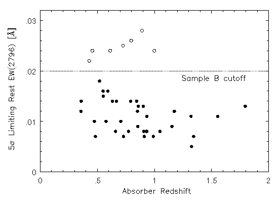
FIG. 3.3 --- The rest-frame equivalent width detection limit (5-sigma) verses absorber redshift. The detection level of Sample B is fairly uniform with redshift; a Spearman-Kendall non-parametric test did suggest a weak anti-correlation, but it is negligible. A correlation in the limiting equivalent width is undesirable because it holds the potential of introducing a bias into the analysis of redshift evolution in the absorption profiles.
For the analysis of the absorption properties and of the VP parameters, it is preferable that each system in the survey be observed to some uniform equivalent width threshold. In particular, this gives a well defined upper limit to the sensitivity level probed in each absorbing system. Since, for a given absorption system, the sensitivity remains virtually unchanged across a given absorption profile, it is not necessary to map out the sensitivity of the survey in velocity space (using a function analogous to the redshift path density). Thus, the sample for further study is selected based upon the equivalent width detection threshold. In Figure 2.1 through Figure 2.24, the 5-sigma EW(rest) limit of the Mg II 2796 transition is presented for each system. The top panels show the feature identifications and the lower panels show the EW(rest) limits as a function of wavelength. The full velocity spread presented in these figures is nominally +/- 500 km/s.
The second reason for selecting the cutoff at 0.02 A was based upon the simulations (Chapter 4). Though not presented therein, simulations with a 0.03 A EW(rest) cutoff were compared to those with 0.02 A and 0.01 A cutoffs. Both the column density completeness limit (for a 99% detection rate) and the accuracy of the resulting VP parameters (following full VP decomposition of the spectra) are strong functions of the limiting EW(rest).
It would also be preferable if the redshift range observed was sampled uniformly. Achieving this goal is nearly impossible, since the selection criteria of systems is highly dictated by the brightness of the QSOs available on the night of the observations. As seen in Figure 3.1, the distribution of systems in redshift drops rapidly for z > 1. Note that all z > 1 systems are included in Sample B. In the final analysis, it will be important to understand if measured redshift evolution in any given absorption property is a result of a selection bias. For one, four of the systems at z > 1.2 have the four largest equivalent widths (EW(rest) > 1.8 A). This is a definite selection bias that occured during the course of the observations. The upper left panel of Figure 3.4 (explained below) shows EW(rest) verses redshift. It is clear that the z > 1 - EW(rest) < 1.8 and the z < 1 - EW(rest) > 1.8 quadrants of the diagram have not been sampled. An extension of the current study would be required to better understand how absorption properties obtained from high resolution spectra are distributed with redshift. There are reasons to believe that the z < 1 - EW(rest) > 1.8 quadrant is relatively underpopulated (Bergeron et al. 1994; SS92; Petitjean & Bergeron 1990), based upon low and medium resolution studies. It is possible that if clear correlations are found between absorption properties that are not sensitive to spectral resolution (i.e. EW(rest), DR, and total omega(v)) and absorption properties obtained at high resolution (i.e. number of VP components and their velocity clustering), then indirect inferences might be drawn from the available large lower resolution databases.
3.3 DISCUSSION OF INDIVIDUAL SYSTEMS (BY QSO)
- Q 0002+051
- Q 0058+019
- Q 0117+212
- Q 0420-014
- Q 0450-132
- Q 0454+036
- Q 0454-220
- Q 0823-223
- Q 1101-264
- Q 1148+384
- Q 1206+456
- Q 1213-003
- Q 1222+228
- Q 1225+317
- Q 1241+174
- Q 1248+401
- Q 1254+044
- Q 1317+274
- Q 1329+412
- Q 1354+193
- Q 1421+331
- Q 1548+093
- Q 1622+235
- Q 1634+706
- Q 2128-123
- Q 2145+064
3.4 EXPLORING THE ABSORPTION PROPERTIES
Trends of gas absorption properties with other system properties (i.e. cloud velocities, internal velocity spreads of the blended "cloud" components, or system redshifts) provide new clues to the physical nature of the absorbing gas. Monotonic "correlations" between properties determined solely from high resolution spectra may reveal fundamentally new information about the absorbing gas. On the other hand, correlations of properties that are roughly independent of the spectral resolution with properties determined from high resolution spectra may provide long sought insights into or confirmations of inferences based upon larger low resolution surveys.
There is a great deal of scatter in the absorption properties. Furthermore, the probability distribution functions from which the properties can be thought to have been drawn are unknown. Thus, when searching for possible relationships between various quantities, it is best to perform simple non-parametric tests for trends. Then, statistically significant trends can be further investigated for possibly having been drawn from an assumed and well defined probability distribution function, which can be parameterized (i.e a linear relationship).
3.4.1 Spearman and Kendall Non-Parametric Tests
The Spearman rank order coefficient, r_s, and the Kendall Tau, tau_k, are both quantities computed from the ranks or relative ranks of data pairs. The probability distribution functions from which these ranks are drawn are well understood, so that the significance level to which the hypothesis of no correlation (null hypothesis) is satisfied can be computed. These two statistical tests are described in Press et al. (1992).
For the Spearman test, each data point, x_i, is replaced by the value of its rank among all other x_i's in the sample. The same is done for the y_i. The resulting list of ranks is thus drawn uniformly from the integers between 1 and N, where N is the number of data points. The significance level, P_s, is computed from the number of standard deviations, N-sigma, by which the sum-squared difference of x and y ranks deviate from the computed null hypothesis value. The sum-squared difference of ranks is approximately normally distributed. Thus, the significance level is the complementary error function evaluated at N-sigma/sqrt(2).
The Kendall test actually invokes relative ranking of the data. The data are broken into pairs; a pair is "concordant" if the relative ranking of the two x's is the same as the relative ranking of the two y's. A pair is discordant if the relative ranking of the x's is opposite that of the y's. The Kendall Tau is computed from the number of concordant and discordant data pairs. Kendall's Tau has a zero expectation value for the null hypothesis, and its variance is also approximately normally distributed. The confidence level, P_k, is also given by the complementary error function evaluated at N-sigma/sqrt(2), where N-sigma is the number of standard deviations by which tau_k deviates from zero.
3.4.2 Overall Absorption Properties
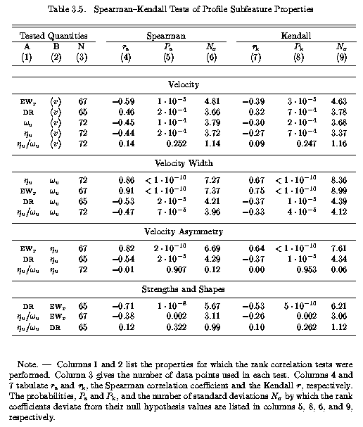
Spearman and Kendall non-parametric rank correlation tests were performed on all Sample B quantities presented in Table 3.1 and Table 3.2. Results for the overall system properties and the subsystem properties are presented in Table 3.4 and Table 3.5, respectively.
In the upper portion of Table 3.4, the tests for correlations of absorbing properties with redshift are presented. In the lower portion of Table 3.4, selected tests for correlations between absorbing properties are tabulated. Also tabulated are tests for correlations of the system redshift, number of subfeatures, and number of VP components with the EW(rest) of the spectrum. These latter tests are to discern if the non-uniform sensitivity of the spectra is introducing bias into the other tests.
Table 3.4
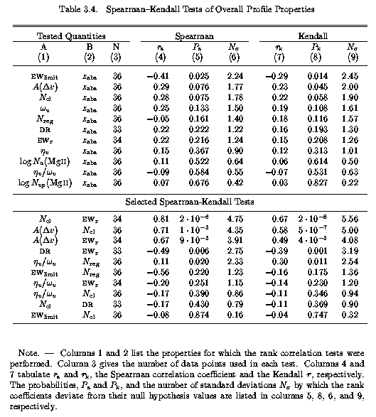
Table 3.5
The tests are listed in order of increasing P_k, that is in order of decreasing likelihood that the null hypothesis is not satisfied. If the criterion that the data are inconsistent with the null hypothesis to the 99.9% confidence level is adopted, then "clear" correlations can be claimed only if P < 0.001. For data that exhibit the level of scatter seen in absorption properties shown in Figure 3.3 through Figure 3.12 such a stringent criterion is required, especially for fewer than 50 data points.
Note that the tests yield P = (P_s,P_k) = (0.025,0.014) for the limiting EW(rest) verses redshift. As illustrated in Figure 3.3, the Sample B limiting equivalent widths do not show a clear trend with redshift apart from a few points that are driving the correlation coefficients to the N-sigma ~2.4 level. The same test on a sample for which the less stringent cutoff limit 0.03 A was applied yielded P = (0.001,0.001). It is probable that an EW(rest) cutoff at 0.03 A would have resulted in biased results with redshift.
In Figure 3.4, selected absorption properties are plotted against absorber redshift. Plotted are rest-frame equivalent width, EW(rest), the median deviation of VP cloud velocities, A(Dv), the absolute value of the shape parameter, | eta(v)/omega(v) |, and the number of clouds per system, N_cl. It is important to remember that the z > 1 portion of the diagrams are under sampled with respect to the z < 1 portions, and that there is a biasing toward large EW(rest) at z > 1.3. Even so, the correlation tests do not allow a rejection of the null hypothesis to the adopted confidence level. Except for | eta(v)/omega(v) |, the same tests on the full sample, Sample A, yielded probabilities more suggestive of correlations, but none yield P<0.01. The lowest probability is for A(Dv), which is accentuated by the weakest systems (N_cl = 1, A(Dv) = 0) at z < 1. The interesting data are the two z < 1 systems with A(Dv) ~150 km/s. These are the Q 1206+456 at z = 0.9276 system and the Q 1254+044 at z = 0.5194 system, respectively. Both systems exhibit a high velocity kinematic subsystem. That two out of 27 systems are seen with these characteristics crudely implies that less than 10% of all z < 1 systems will be observed to have these very high velocity kinematic subsystems to a limiting EW(rest) of 0.02 A.
Figure 3.4
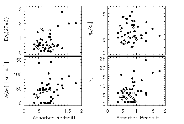
FIG. 3.4 --- The redshift distribution of selected overall absorption properties taken from those presented in Table 3.4 --- (upper left) the rest-frame equivalent width --- (lower left) the median deviation of VP cloud velocities --- (upper right) the "shape parameter" --- (lower right) the number of clouds per system. The solid points are taken from Sample B and the open points are taken from the full sample (those rejected from Sample B). Based upon Spearman-Kendall tests on Sample B, none of the illustrated absorption properties are inconsistent with no correlation with redshift above the 2-sigma significance level. The trends that are present are primarily due to the selection of large equivalent width systems at the higher redshifts. Thus, any suggestion of weak correlations in these data likely results from selection effects.
In Figure 3.5, a small selection of overall absorption properties is presented. These quantities are taken from Table 3.4 to illustrate a range of correlation significance levels. It was important to verify that the number of VP components, N_cl, shows no correlation with the equivalent width limit of the spectra. Indeed, this was verified to a high degree as can be seen in the last entry of Table 3.4 and in the lower left panel of Figure 3.5. Had a correlation been found, it would place serious doubts on the results of the VP decompositions. It is also found that the number of subfeatures, or subsystems, is not correlated to the equivalent width limit of the spectra. With little doubt, it can be claimed that any conclusions based upon the subsystems or the number of clouds are not weakened non-uniformity in the signal to noise.
Figure 3.5
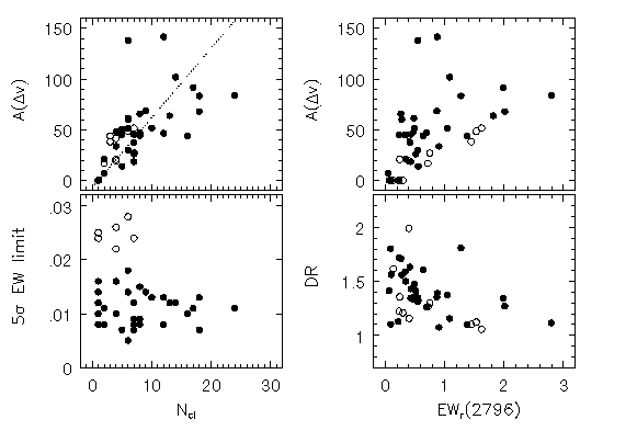
FIG. 3.5 --- A small selection of overall absorption properties taken from Table 3.5 to illustrate a range of correlation significance levels --- (upper left) the median deviation of VP cloud velocities verses the number of VP clouds --- (lower left) the equivalent width detection level verses the number of VP clouds --- (upper right) the median deviation of VP cloud velocities verses equivalent width --- (lower right) the Mg II doublet ratio verses equivalent width. The solid points are taken from Sample B and the open points are taken from the full sample (those rejected from Sample B). The effects of lower signal to noise ratios on the number of VP components, N_cl, can be seen in the lower left panel. The dotted line represents a maximum likelihood fit to the "spread" of cloud velocities as a function of the number of clouds. Note that A(Delv) = 0 at N_cl = 1 by definition.
The highest confidence levels (lowest values of the probabilities) that the null hypothesis can be ruled out, are seen for the N_cl verses EW(rest) test and for the A(Dv) verses N_cl test. Not surprisingly, A(Dv) is correlated with EW(rest) to the required confidence level. Note also, that the Mg II doublet ratio is anti-correlated with EW(rest) (this is confirmation that the correlation tests are fairly useful, since this particular test had better come up with a non-null result). Illustrated in Figure 3.6 is a correlation of the number of clouds with EW(rest). This correlation was first recognized by Wolfe (1986) and by York et al. (1986), and later demonstrated by Petitjean & Bergeron (1990) and Churchill, Steidel, & Vogt (1996). Following those authors, a linear relation has been fit to the data, excluding the cross hatched points. These points are Q 0450-132 at z = 1.1746, Q 1213-003 at z = 1.5541, Q 1225+317 at z = 1.7948, and Q 1213-003 at z = 1.3201, in increasing number of VP components. It is likely that N_cl has been underestimated for these systems, possibly by as much as a factor of ~1.5 (see Figure 4.13). A correction factor of this magnitude would place these points closer to the fitted line. An effect due to the signal to noise in the spectra can be seen, as well. Note the open circles, which have EW(rest) > 0.02 A limits (corresponding to a signal to noise ratio S/N ~ 22 per three pixel resolution element). It is likely that the number of VP components has also been underestimated for these systems.
In Figure 3.6, two linear fits to the Sample B data are shown. The dash-dot line is a maximum likelihood fit with slope m = 0.076 +/- 0.004 and the dotted line is a chi^2 minimizing fit with slope m = 0.093 +/- 0.007, where the reduced chi^2 = 0.9. Errors in both EW(rest) and N_cl were included in the chi^2 fit, which likely explains the large slope in view of the assumed sqrt(N) uncertainties in the cloud numbers (which is not very appropriate because the uncertainties in the N_cl are not normally distributed-- the N_cl are systematically underestimated due to component blending). Thus, the maximum likelihood slope is probably a more realistic result. In addition, this value is comparable to the value 0.070 found by Churchill, Steidel, & Vogt (1996). This slope is significantly smaller than the value ~0.35 obtained from the Petitjean & Bergeron (1990) fit to 30 km/s resolution spectra.
Figure 3.6
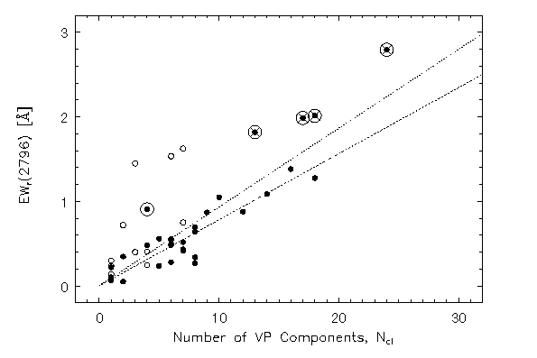
FIG. 3.6 --- The Mg II 2796 equivalent width is strongly correlated to the number of VP components, or clouds. The solid points are taken from Sample B and the open points are taken from the full sample (those rejected from Sample B). The four points with cross hatches are, Q 0450-132 at z = 1.1746, Q 1213-003 at z = 1.5541, Q 1225+317 at z = 1.7948, and Q 1213-003 at z = 1.3201, in increasing number of VP components. These systems exhibit highly saturated broad profiles. These four systems were not included in either the maximum likelihood fit (dash-dot) nor the chi^2 minimizing fit (dotted). See text for details. The outlier at (4,0.91) is from the Q 0117+212 system at z = 0.5764, which is also a highly saturated profile for which the number of components is likely under estimated.
It is useful to ask if the internal velocity spread can be inferred from the value of EW(rest), which can be measured in low resolution spectra. A maximum likelihood linear fit was obtained to the A(Dv) verses N_cl data, for which a slope of 6.72 +/- 0.76 was obtained. However, as can be seen in Figure 3.4, the data exhibit increased scatter for A(Dv) > 40 and N_cl > 10. The systems with N_cl greater than 15 are dominated by the broad saturated systems. For these, N_cl is likely a lower limit, based upon the VP fitting simulations (see Chapter 4). A system for which N_cl is underestimated would properly occupy a position down and to the left of where it has been plotted; this tends to increase the scatter with respect to the "correlation line". It is clear that A(Dv) is sensitive to somewhat extreme kinematics that cannot be discerned simply from the number of VP components. Since the EW(rest) is correlated with N_cl, it follows that the average kinematic spread cannot be inferred from EW(rest) with confidence. Primarily, this is due to saturation/blending on one extreme and due to the chance presence of high velocity subsystems that do not contribute much to the value of EW(rest) on the other.
In Figure 3.7, the histogram distributions of N_cl, EW(rest), omega(v), and | eta(v)/omega(v) | are presented. The shaded distributions are the Sample B systems, and the unshaded distributions are the full sample presented in Table 3.1. What is apparent is that the Sample B distributions are fairly flat and that the low signal to noise systems cluster at smaller N_cl, EW(rest), omega(v), and | eta(v)/omega(v) |. In the case of EW(rest), these systems are clustered at low redshift, and this may be an artifact of the redshift-EW(rest) distribution. For the other absorption properties, it appears that some information from the absorption profiles is truly "missed" for the limit EW(rest) > 0.02 A. In these systems there may be lurking undetected undulations in the profile shapes (i.e. asymmetries, VP components) and/or kinematic subsystems (also see Figure 3.12, from which one can infer that there are roughly as many subsystems in the range 0.01 < EW(rest) < 0.02 A as there are in the range 0.02 < EW(rest) < 0.03 A).
Figure 3.7
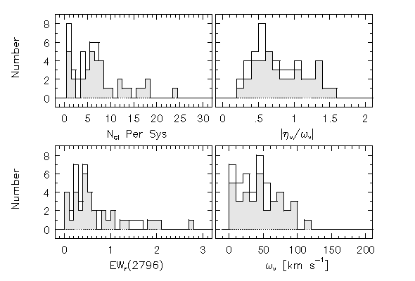
FIG. 3.7 --- Histogram distributions of selected overall absorption properties --- (upper left) the number of VP components per system --- (lower left) the equivalent width --- (upper right) the profile asymmetry per unit width (shape parameter) --- (lower right) the profile velocity width. The thick line histogram shows the full sample presented in Table 3.1, and the shaded region gives the distribution of Sample B.
3.4.3 Subfeature Absorption Properties
Just exactly what are the absorbing subfeatures, or kinematic subsystems, as they have been defined for this work? Is it meaningful to segregate the overall profiles into distinct absorption subsystems simply based on there being a stretch of continuum between two absorption profiles within a predefined velocity range that are detectable down to some predefined sensitivity level? Can the notion of subsystems be taken a step further-- can they be treated as a population of absorption systems in their own right from which a deeper appreciation of the overall systems can be gleaned? If this line of questioning is affirmed, then it may be that these subsystems will provide insights into the ionization conditions, spatial distributions and kinematics of different sub-populations of absorbing clouds (i.e perhaps optically thin clouds can be inferred to be located in galactic halos, etc). In particular, trends of subsystem absorption properties with their velocities, or with the galaxy properties [when these become available for a larger sample than that studied by Churchill, Vogt, & Steidel (1996)], may provide clues for answering the above questions. Perhaps these subsystems may actually be isolated absorbing "clouds" or spatially separated absorbing regions within galaxies.
Recall that the velocity zero point for all systems is the optical depth mean of the Mg II 2796 profile. Thus, the subsystems at small velocities will tend to have the largest optical depths and will systematically have larger EW(rest), smaller DR, and greater omega(v). These can be understood entirely in terms of the definition of the velocity zero point. However, it is not clear how these absorption properties will be distributed , nor how they will be distributed in velocity space.
Figure 3.8
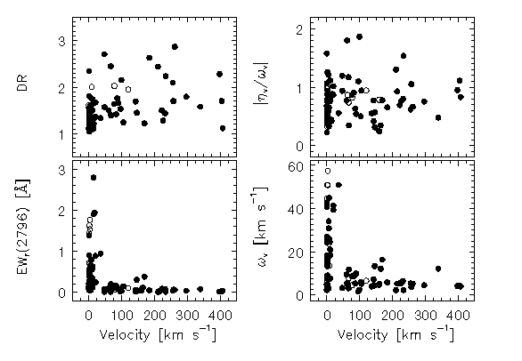
FIG. 3.8 --- A selection of subfeature absorption properties verses velocity for which correlation tests were performed (see Table 3.5) --- (upper left) the doublet ratio --- (lower left) the equivalent width --- (upper right) the shape parameter --- (lower right) the velocity width. Most telling is the strong clustering of omega_v < 10 km/s and of EW(rest) < 0.2 A for v > 40 km/s.
In Figure 3.8, the subfeature DR, EW(rest), omega(v), and | eta(v)/omega(v) | are presented verses velocity in a scatter plot. These properties are listed in Table 3.3. Spearman and Kendall non-parametric rank correlation tests were performed for all Sample B subfeature quantities. In the upper portion of Table 3.5, the tests for correlations of absorbing properties with velocity are presented. At first glance it looks as if all tested properties, except the shape parameter, show significant trends with increasing velocity. However, there is an over representation of subsystems with v=0 km/s. In fact, for every absorption system, there is a subsystem with v=0 km/s because of the velocity zero point definition. The non-null result for the correlation tests occur because these subsystems cluster, as predicted.
The histogram distributions of selected subfeature absorption properties are presented in Figure 3.9. The upper left panel shows the doublet ratios, the lower left shows the equivalent widths, the upper right shows the subfeature shape parameters, and the lower right shows the subfeature velocity widths. It is interesting to compare these distributions with those of the full features in Figure 3.7. What is most striking is how peaked the the equivalent widths and the velocity widths are at small values for the subsystems.
Figure 3.9
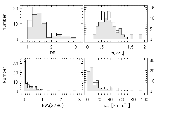
FIG. 3.9 --- Histogram distributions of selected subfeature absorption properties --- (upper left) the doublet ratios --- (lower left) the equivalent widths --- (upper right) the subfeature asymmetries per unit width (shape parameter) --- (lower right) the subfeature velocity widths. The thick line histogram shows the full sample presented in Table 3.3, and the shaded region gives the distribution of Sample B.
In
All subsystems with v > 40 km/s have been culled into a separate
sample. The histogram distributions of the subsystem DR,
EW(rest), omega(v), and | eta(v)/omega(v) |, are
again illustrated in
Figure 3.11.
However, this
figure includes only Sample B (grey shade). The black shaded
histogram is the population of v > 40 km/s subsystems.
Though DR greater than two is unphysical, the doublet ratios of the
v > 40 km/s subsystems are suggestive of optically thin gas for the
most part. Roughly 80% of subsystems with
EW(rest) < 0.2 A are accounted for by
v > 40 km/s subsystems. Most of these
v > 40 km/s subsystems have omega(v) < 10 km/s. Taken
together, these results are suggestive that these subsystems are a
subpopulation characterized first and foremost by their velocity
with respect to the optical depth mean of the overall system.
As illustrated in
Figure 3.12,
there is no clear turnover
in the EW(rest) distribution of the v > 40 km/s subsystems.
As
Figure 3.12
is presented, the counts in each bin have
not been corrected for partial contributions [a system with a
5-sigma detection limit of 0.0075 A samples only 50% of the
smallest bin (0.005-0.01 A)].
That there are no counts in this smallest bin is consistent with
no turnover in the distribution once a correction is applied.
Of the observed 33 systems, 13 have 5-sigma detection limits
that partially sample this smallest bin (one of them samples the entire
bin). If these 13 are weighted by the fraction of the bin each
samples, then there are effectively ~5 systems. If the
distribution is flat, the expected number of counts in any bin is
given by the average counts in bins with EW(rest) >
0.02 A, where the sample is complete. The average number of
counts between 0.02 < EW(rest) < 0.05 A is ~2.
Thus, 2(5/33)=0.3 counts, which is consistent with the observed null
detection, are predicted in the 0.005-0.01 A bin.
The apparent optical depth method (Savage & Sembach 1991}) for obtaining the
N_a(v) profiles is well suited for quantifying the degree of
unresolved saturation at each velocity location along the absorption
profiles. It also provides a very useful technique for obtaining the
integrated column density, N_a, especially for doublets or
transitions of a given ion for which the f are a factor
of two different. An example of inverted profiles are presented in
Figure 3.13
for three systems. These profiles illustrate
the technique presented in
Section 2.5.
Shown are the N_a(v) profiles for the Mg I transition and the
Mg II doublet from the
Q 1213-003 at z = 1.3201 system.
Also shown are the Mg II doublets from the
Q 1101-264 at z = 0.3563 system, and
from the Q 0117+212 at z =
1.0479 system. Note the heavy saturation in Mg II for the
Q 1213-003 system,
where the 2803 data give a more accurate
lower limit of N_a(v). Also note the discrepancy in the data for
the Q 1101-264 system. The
2803 transition is likely
blended with a Ly-alpha absorption line, given the level of confusion in
the spectrum over the observed wavelength region.
It is also interesting to compare N_a with the integrated VP
column densities, N_vp. In
Figure 3.14
log N_a(Mg II) is plotted verses log N_vp(Mg II).
Though the number of data points is small, it
appears that column density regimes at which these two methods break
down from the tight correlation are not identical. In other words,
small fractional errors are still obtained for the log N_vp(Mg II)
up to 14.0 cm^-2 or higher when the log
N_a(Mg II) are only lower limits at 13.5 cm^-2. A deeper
appreciation of this figure would require studying this relationship
for simulated spectra. This particular issue was not studied in
Chapter 4.
Clearly, however, a power law fit to the
distribution of system column densities would result in a relatively
steeper power if one were fitting the N_a. Thus, inferring the
system integrated column density distribution from the VP column
densities is likely to recover a power law slope more commensurate
with the true distribution.
Figure 3.10
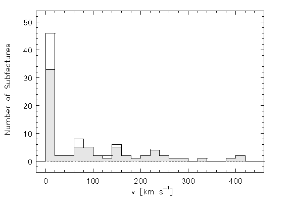
FIG. 3.10 ---
Histogram distribution giving the number of subfeatures per
20 km/s bin. The thick line histogram shows the full
sample presented in
Table 3.2,
and the shaded region
gives the distribution of Sample B. Out of 33 absorption systems,
there are 39 subfeatures with v > 20 km/s, from which one can
estimate that, on average, there is more than one higher velocity
subsystem per absorber with equivalent widths greater than
the sample completeness.
Figure 3.11
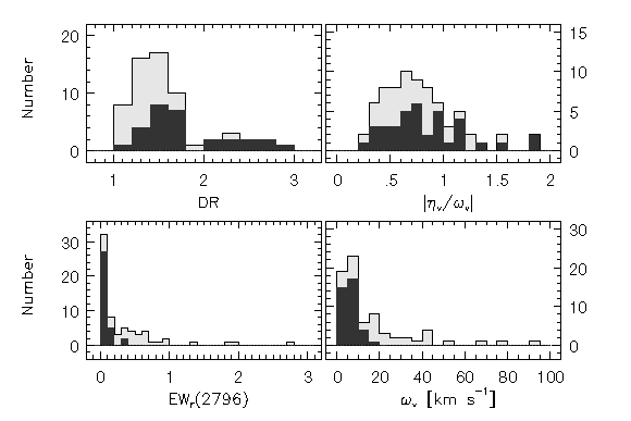
FIG. 3.11 ---
Based upon the subfeature velocity distribution (see
Figure 3.10),
the properties of subfeatures with
v > 40 km/s were binned as a separate population of absorbers
--- (upper left) the doublet ratios --- (lower left) the equivalent
widths --- (upper right) the subfeature asymmetries per unit width
(shape parameter) --- (lower right) the subfeature velocity widths.
The lightly shaded histograms are the full Sample B (all velocities) and
the solid filled histograms are the v > 40 km/s subpopulation.
Though DR greater than two is unphysical, these doublet ratios are
suggestive of optically thin gas, where as very few v > 40 km/s
subfeatures are optically thick.
Figure 3.12
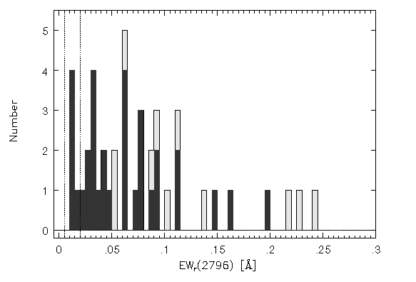
FIG. 3.12 ---
The subfeature rest-frame equivalent widths binned at 0.005 A.
The region of partial completeness
0.005 < EW(rest) < 0.02 A) is marked by the vertical
dotted lines. The lightly shaded histogram is the full Sample B (all
velocities) and the solid filled histogram is the v > 40 km/s
subpopulation. Note that all EW(rest) < 0.05 A
subfeatures have
v > 40 km/s. Though the statistics are small, there is no clear
evidence for an EW(rest) cutoff of so called "satellite" lines in
Mg II absorption systems. This is particularly evident in view
of the fact that, for EW(rest) < 0.02 A, the sample is
not complete.
3.5 COMPARING INTEGRATED AOD AND VP COLUMN DENSITIES
Figure 3.13
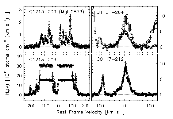
FIG. 3.13 ---
The apparent column densities, N_a(v) for three selected
systems. The left two panels are N_a(v) for the
Mg I transition (upper) and for the Mg II doublet (lower) from the
Q 1213-003 at z = 1.3201 system.
The upper right panel is the Mg II doublet from the
Q 1101-264 at
z = 0.3563
system, and the lower right panel shows Mg II from the
Q 0117+212 at z = 1.0479 system.
The error bars are the 1-sigma
uncertainties. For the Mg II doublets, open circles are the
2803 transition and boxes are the 2796
transition. The uncertainties are not shown for the saturated pixels,
which give a lower limit to N_a(v)$. Note the discrepancy in the
Q 1101-264 profiles.
The 2803 transition is likely blended
with a Ly-alpha absorption line.
Figure 3.14
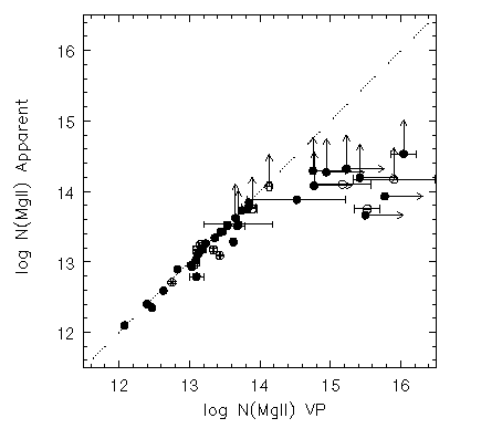
FIG. 3.14 ---
The full Mg II 2796 profile apparent column densities
verses the VP decomposition column densities (see
Table 3.2).
The solid points are taken from Sample B and the open points are
taken from the full sample (those rejected from Sample B).
The formal uncertainties are shown, but are often the size of
the data points. Lower limits are given by the arrows (for the VP
column densities, a lower limit is shown in the case where the
fractional error is > 1).
There is a clear breakdown of the correlation at a VP column
density of log N ~ 14.5 cm^-2, corresponding to an apparent
column density where unresolved saturation sets in, log N_a ~
13.5 cm^-2.