2. DATA REDUCTION AND ANALYSIS
2.1 DATA REDUCTION
The HIRES data were reduced with the IRAF (IRAF is distributed by the National Optical Astronomy Observatories, which are operated by AURA, Inc., under contract to the NSF.) Apextract package for echelle data. The detailed steps for the reduction are given in Churchill (1995).
For each night at the telescope, a series of ~10 bias frames (which will be denoted as [BIAS]) were obtained. For each setting of the HIRES spectrograph, a series of ~10 quartz lamp frames (denoted [FLAT]) were obtained using a decker that had twice the projected spatial dispersion as the program decker (see Table 1.1). Use of the "wide" decker results in high signal from the quartz lamp where the sky regions of the spectra fall on the detector. This technique allows the sky background to be flatfielded while preserving the color sensitivity of the quantum efficiency in each pixel. In almost all cases, three object frames (denoted [RAW], since they are uncalibrated) of each QSO were obtained. By splitting the total exposures into thirds, cosmic rays could be removed in a systematic way. Thorium Argon (Th-Ar) lamp frames, used for wavelength calibrating the reduced spectra, were obtained before and after every QSO observation. Dark frames were obtained on the January run, but were not used since the dark current was seen to be negligible. Thus, the set of calibration frames for each un-calibrated data frame [RAW] consisted of N_B bias frames [BIAS], and N_F flat field frames [FLAT], and a series of Th-Ar frames.
2.1.1 Instrumental Calibration
Each observed [RAW] data frame was overscan subtracted, bias frame corrected, and flatfielded in the standard fashion, a simple series of additive and multiplicative calibration steps. The desired data frame ([DATA]) is convolved with instrumental "information" according to

where OS_RAW is the overscan of [RAW], the "flat" term is a convolution of the transmission function and quantum efficiency, and the "scatter" term is the scattered light from within the spectrograph that is detected by the CCD. Since the electronics were stable, the noise in the individual [BIAS] and [FLAT] frames was reduced by averaging them with "cleaning" algorithms according to

The IRAF tasks zerocombine and flatcombine were used, respectively, both with the "minmax" pixel rejection mode since cosmic rays were not a contributing noise source in these short exposure frames. This rejection mode allows one to define the number of pixels that will be retained for the averaging computation so that the rejection statistics for each pixel are drawn from the same sample size. The cleaned [FLAT] frame was then normalized to unity using the apnormalize task. The scattered light was modeled using the task apscatter, which simply fits a two-dimensional smoothed surface to the inter-order regions of the echelle format on the CCD. This surface is computed for each [RAW] frame (uncombined QSO exposures) and output as a scattered light frame ([SCATTER]). The scattered light was often negligible. Finally, each calibrated data frame [DATA] was obtained by

using the IRAF task ccdred.
2.1.2 Cosmic Ray Removal and Calibration Uncertainties
At this point, the [DATA] frames were converted to units of electrons by multiplying the DN in each pixel by the system gain. This is a necessary step in order to properly account for the Poisson fluctuations, which are proportional to the electrons measured and not to the artificial DN values output by the HIRES data acquisition system. Cosmic rays and noise were removed by averaging the [DATA] frames for each QSO using the IRAF task imcombine. This technique was possible only because the HIRES spectrograph was extremely stable between exposures. By interpolating the two-dimensional wavelength solutions of the Th-Ar lamps taken over the course of a night, it was found that no systematic shift (using ecreidentify) occured in the cross disperser and echelle settings within the RMS uncertainty of the pixel verses wavelength solutions. Thus, the Th-Ar lamps taken throughout the night were added together, and this single frame was eventually used for the wavelength calibration. For the data frame averaging, the imcombine task was used with the "crreject" mode, which uses a sigma rejection method based upon the readnoise added in quadrature with a simple Poisson fluctuation model of the counts in each pixel. A rejection sigma of three was used; for a given pixel, if the value in a given frame was 3-sigma above the average value taken from all input frames, then that frame was rejected from the final average (single iteration). This technique resulted in a virtually perfect removal of all cosmic rays and yielded a working frame with reduced noise characteristics. A "sigma frame" ([SIGMA]) for each QSO frame was output by imcombine, which was taken to be the 1-sigma uncertainty in the value of any pixel due to the entire calibration process described above.
2.1.3 Optimized Extraction of the Spectra
[This Subsection is Abridged] The spectra were "extracted" using the optimal routines of Horne (1986) and Marsh (1989). The algorithm is designed to best determine the fraction of flux that falls into each dispersion pixel (at every wavelength) of the spectrum. This is achieved by optimally weighting the flux values in each cross dispersion pixel used in the extraction sum. This minimizes statistical noise and maximizes photometric accuracy.
To account for the noise added during the instrumental calibration processing, the [SIGMA] frames output by the imcombine task were also "extracted" using the aperture models for their respective QSO frames. To obtain the final sigma spectrum for each QSO spectrum, these "calibration sigma spectra" were then added in quadrature to the "extraction sigma spectra" output by the optimal extraction task apall.
The final reduction step was to "attach" the wavelength solution of the added Th-Ar frames. The wavelengths were calibrated to vacuum using ecidentify. The term "attached" is used here because the spectra were not resampled, or linearized, so that the absorption profile shapes would not be altered. The resampling process involves inverting the wavelength verses pixel solution followed by a flux conserving interpolation of the I(lambda) data values. This introduces correlated errors between the I(lambda) that are difficult to treat.
The heliocentric velocity offset was computed for each spectrum and was applied at the time that each was converted to ASCII format. The IRAF task rvcorr was fed a list that included the right ascensions, declinations, and UT dates (half-way point of the integrations) of the QSOs. Output were the HJD dates and the heliocentric velocity offsets.
2.2 ANALYSIS OF THE SPECTRA
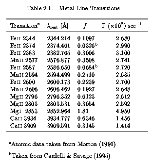
The final calibrated spectra and the Voigt profile models are presented in Figures~\ref{fig:vpfits}-\ref{fig:endvpfits}. All further processing of these calibrated spectra was performed using personalized codes and data formatting in the Unix environment and using SunOS Fortran 77. Since this is a study of the transitions arising from ions in "low" ionization gas, only the transitions given in Table 2.1 were searched for each system. These transitions were selected primarily because of their relatively large abundances (based upon solar), their strong oscillator strengths, and the fact that rest-frame transition wavelengths below 2300 A fell below 4000 A where the HIRES sensitivity drops dramatically for z_abs < 0.7 systems (there was little point to go bluer).
The search strategy for these ions in each system was as follows. First, the complete echelle order(s) containing the Mg II 2796, 2803 doublet was converted to ASCII format and continuum normalized. The ASCII format spectrum consisted of seven columns, (1) wavelength, lambda (2) velocity, v, (3) normalized flux, I/I_c, (4) normalized errors, sigma_I/I_c (5) flux, I, (6) continuum fit, I_c, and (7) the errors sigma_I. An absorption feature identification algorithm, called ewregion (described below), was run on the spectrum, and the wavelength region over which the Mg II 2796 profile was detected. Then, the systemic absorption redshift of the Mg II 2796 profile was computed, as described in Section 2.2.3. For each system, this is the adopted systemic redshift (listed in Table 3.1) for all further analysis, and it gives the profile velocity zero points. Finally, the regions of the QSO spectrum corresponding to the target ions in Table 2.1 were converted to ASCII format over a region +/- 500 km/s from the transition's systemic redshifted wavelength (or larger if the features of the Mg II profiles extended to greater velocities). The ewregion code was then run on each transition spectrum, simply for the purpose of determining if significant absorption was present and for computing the limiting detectable equivalent width as a function of velocity. If a given transition spectrum had no detected features, then no further processing was performed on the spectrum. Often, the absorption profiles of a given system are complex, suggestive of a multi-subcomponent structure. It is a slight misnomer to label these profiles as absorption lines. For the following analysis, a feature designates the entire absorption profile for each transition. Some features may be subdivided into regions, which can be thought of as subfeatures separated by continuum (see Figure~\ref{fig:ewlims} for examples of how subfeatures are defined and numbered). A subfeature may also show complex subcomponent structure. The term absorption "line" is reserved for the cases in which a feature or subfeature exhibits no evidence for being comprised of subcomponents. In effect, each subcomponent in a subcomponent analysis could be considered a "line".
Each subfeature region is defined by an upper and a lower velocity, (v-,v+). The v- and v+ are output by ewregion when it is run on the Mg II 2796 transition. Thus, the velocity interval defining each region is based entirely upon the Mg II 2796 transition. In some cases, a weaker transition of a different ion may not exhibit a detectable subfeature in a given region, say where Mg II is weak. In no case does a transition of any other ion exhibit a subfeature in a velocity interval in which Mg II does not. Thus, each subfeature can be individually analyzed, in that, for each an equivalent width, double ratio, mean velocity, velocity width, and integrated column density can be measured.
The spectrum of each transition was continuum normalized over the +/- 500 km/s region using the IRAF task sfit. The sfit task was selected because it allows interactive selection of the regions of the spectrum to be included or excluded in the fitting process. Thus, absorption subfeatures could be masked during the fitting process, and "bad" pixels could be replaced by the fit itself. These "cleaned" pixels were those with deviations greater than five times 5-sigma) the fitting function RMS residual, following 5 fit-rejection iterations.
Following Sembach & Savage (1992), a Kth order Legendre polynomial of the standard form,

was used, where the c_k are the fitting coefficients, and the P_k are the basis functions of the standard form. In order to properly account for the uncertainties in measured quantities due to the continuum fitting process, it is desirable to use a superposition of orthogonal functions. Then, adding additional terms to the continuum fit increases the error. The goal is to use the lowest order for which the continuum fit is statistically well described. If the fit minimizes the chi^2 statistic,

the F-test (Bevington 1969; Press et al. 1986) provides a means to quantify the significance of an additional term in the fit. For a fit with order k, the F-test is the comparison of the value

with tabulated values of F which give the probability that the additional term does not significantly contribute to the reduction of the chi^2 statistic. Following Sembach & Savage, the 95% significance level was chosen.
An IRAF cl script was written that used the sfit task as a subroutine for the fitting process. In a two-step process, the script allowed the interactive fitting of the continuum, and then automatically iterated the polynomial orders from k = 1 to 5, until the F test was satisfied. In no case was a 5th order polynomial required. In almost all cases, the interactive fit was the same order as that resulting from the automated F-test. In all cases, the F-test result was adopted.
Since the P_k(x) are orthogonal over the range -1 < x < +1, the velocity coordinate of each spectrum was converted to normalized coordinates using a normalization constant,

where v_max is the extreme velocity of a given ASCII spectrum. Whenever possible, the velocity interval of the ASCII spectrum for each transition in a system was the same, to provide uniformity. Since, in almost all cases, the ASCII spectrum of each transition is over a fixed velocity interval, the normalization constant x_s is simply 500 km/s.
Absorption features in the spectra have been identified using the "aperture" method used by Lanzetta, Turnshek, & Wolfe (1987), using a routine called ewregion. Most all subfeatures are well resolved in the sense that their widths are a few to several times greater than the instrumental profile. This technique is not optimal, however, for weak unresolved lines, which are best detected using the instrumental profile weighting technique employed by Schneider et al. (1993) for the HST Quasar Absorption Line Key Project. Such an optimal finding scheme is not well suited for defining blended lines with complex profile shapes, since the instrumental profile in these cases primarily "blurs" the individual subcomponents on a scale small compared to the overall feature.
Each "detection aperture" consists of a small number of pixels that span more than a single resolution element. The observed absorption "equivalent width" of a single pixel is defined as

where I(lambda_j) is the flux in pixel j, I_c(lambda_j) is its fitted continuum level, and Del_lambda_j = (lambda_[j-1] - lambda_[j+1])/2 is the wavelength interval spanned by the pixel. The estimated continuum level is a major source of uncertainty in the measured equivalent width and its contribution requires careful treatment. A proper treatment of the continuum uncertainty should include the fact that the continuum is a smoothly varying function and that any two points are necessarily correlated by the nature of the continuum fitting process. As described by Sembach & Savage (1992), and outlined below, a precisely defined technique can be employed for computing the errors in the observed equivalent width when the full absorption feature spans a non-negligible number of pixels. However, it is not necessary to rigorously compute the correlated uncertainties for the purpose of detecting and identifying absorption subfeatures in the spectrum over only a few pixels. Thus, ewregion does not treat continuum errors, so that the standard deviation in the ew_j are given by

where the sigma_I(lambda_j) are the 1-sigma uncertainties in the I(lambda_j) resulting from data reduction and calibration sources and due to Poisson noise in the QSO flux and sky.
Since the smallest resolved lines are expected to span more than a single resolution element, a "detection aperture" of 2.3 resolution elements (i.e. ~7 pixels) has been chosen. The observed equivalent width of the aperture centered at pixel i and its variance are given by

and

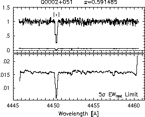
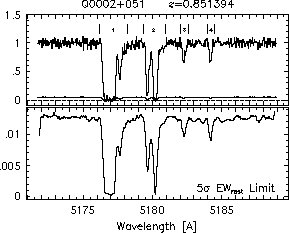
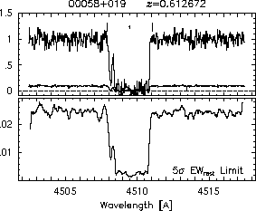
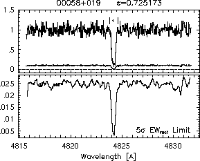
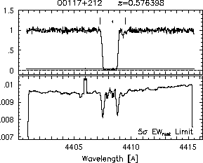
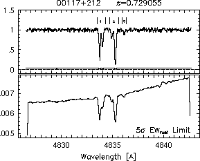
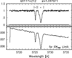
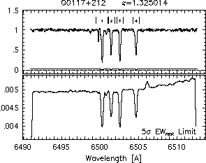
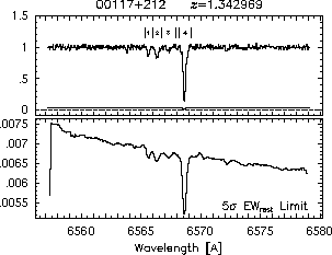
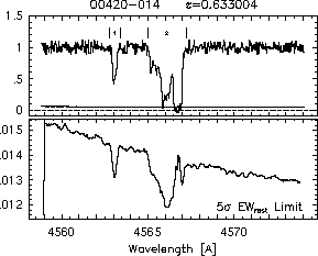
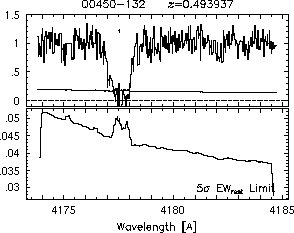
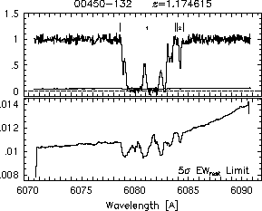
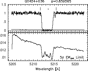
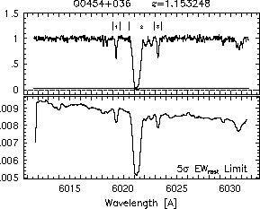
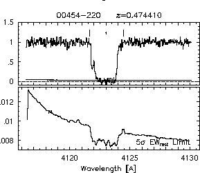
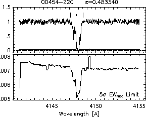
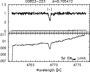
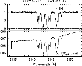
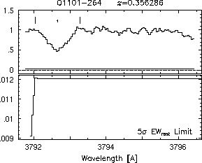
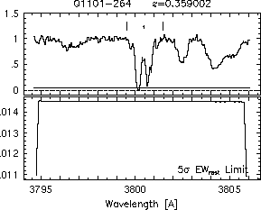
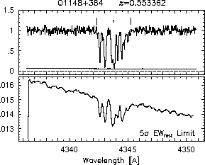
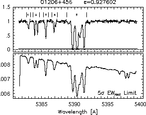
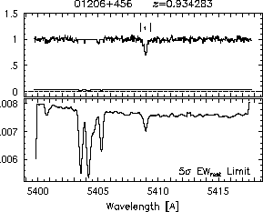
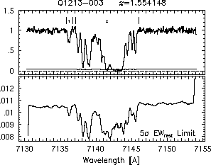
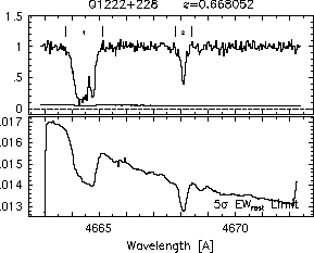
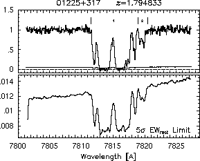
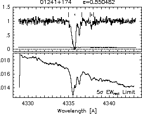
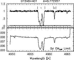
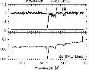
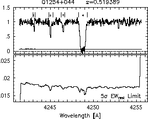
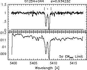
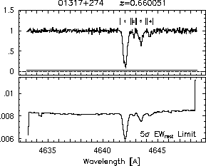
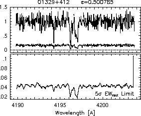
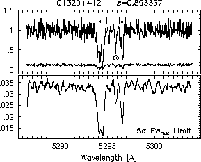
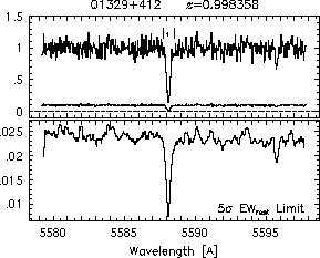
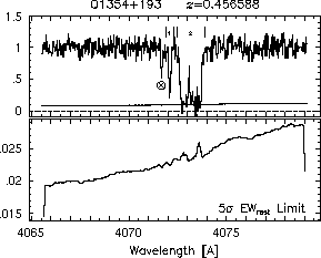
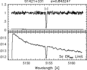
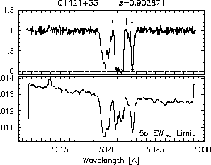
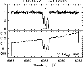
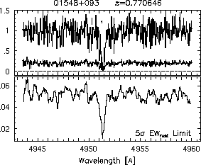
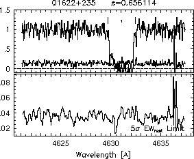
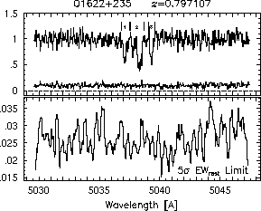
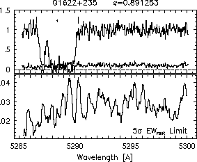
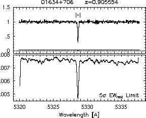
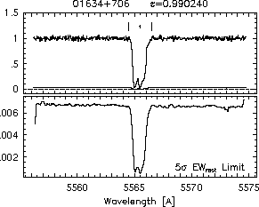
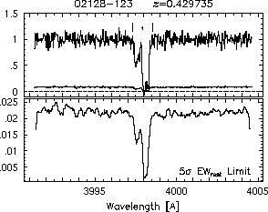
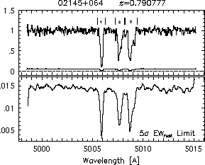
respectively. A significant detection of an absorption subfeature centered on pixel i occurs when EW_i/sigma_[EW_i] > 5. The region over which an absorption feature is detected is defined by its blue-wing edge, lambda-, and its red-wing edge, lambda+. The identified regions are illustrated in Figure 2.1 through Figure 2.48.
Figures 2.1a-b
FIGs. 2.1a-b --- Definition of features and subfeatures, and the 5-sigma detection level. The upper panels show the spectral "regions" (numbered) where the individual subfeatures of the Mg II 2796 transition are found. The lower panels show the 5-sigma equivalent width detection limits.
Figure 2.1c-d
FIGs. 2.1c-d --- Definition of features and subfeatures, and the 5-sigma detection level.
Figure 2.1e-f
FIGs. 2.1e-f --- Definition of features and subfeatures, and the 5-sigma detection level.
Figure 2.1g-h
FIGs. 2.1g-h --- Definition of features and subfeatures, and the 5-sigma detection level.
Figure 2.1i-j
FIGs. 2.1i-j --- Definition of features and subfeatures, and the 5-sigma detection level.
Figure 2.1k-l
FIGs. 2.1k-l --- Definition of features and subfeatures, and the 5-sigma detection level.
Figure 2.1m-n
FIGs. 2.1m-n --- Definition of features and subfeatures, and the 5-sigma detection level.
Figure 2.1o-p
FIGs. 2.1o-p --- Definition of features and subfeatures, and the 5-sigma detection level.
Figure 2.1q-r
FIGs. 2.1q-r --- Definition of features and subfeatures, and the 5-sigma detection level.
Figure 2.1s-t
FIGs. 2.1s-t --- Definition of features and subfeatures, and the 5-sigma detection level.
Figure 2.1u-v
FIGs. 2.1u-v --- Definition of features and subfeatures, and the 5-sigma detection level.
Figure 2.1w-x
FIGs. 2.1w-x --- Definition of features and subfeatures, and the 5-sigma detection level.
Figure 2.1y-z
FIGs. 2.1y-z --- Definition of features and subfeatures, and the 5-sigma detection level.
Figure 2.1aa-bb
FIGs. 2.1aa-bb --- Definition of features and subfeatures, and the 5-sigma detection level.
Figure 2.1cc-dd
FIGs. 2.1cc-dd --- Definition of features and subfeatures, and the 5-sigma detection level.
Figure 2.1ee-ff
FIGs. 2.1ee-ff --- Definition of features and subfeatures, and the 5-sigma detection level.
Figure 2.1gg-hh
FIGs. 2.1gg-hh --- Definition of features and subfeatures, and the 5-sigma detection level.
Figure 2.1ii-jj
FIGs. 2.1ii-jj --- Definition of features and subfeatures, and the 5-sigma detection level.
Figure 2.1kk-ll
FIGs. 2.1kk-ll --- Definition of features and subfeatures, and the 5-sigma detection level.
Figure 2.1mm-nn
FIGs. 2.1mm-nn --- Definition of features and subfeatures, and the 5-sigma detection level.
Figure 2.1oo-pp
FIGs. 2.1oo-pp --- Definition of features and subfeatures, and the 5-sigma detection level.
Figure 2.1qq-rr
FIGs. 2.1qq-rr --- Definition of features and subfeatures, and the 5-sigma detection level.
Figure 2.1ss-tt
FIGs. 2.1ss-tt --- Definition of features and subfeatures, and the 5-sigma detection level.
Figure 2.1uu
FIGs. 2.1tt --- Definition of features and subfeatures, and the 5-sigma detection level.
The redshift of each absorbing system was determined based upon the Mg II 2796 profiles (or the Mg II 2803 profiles when the former were not available). The absorption redshift, z_abs, of each system is defined by

where lambda_sys is median wavelength of the apparent optical depth distribution of the Mg II absorption profile, obtained by solving

where lambda- and lambda+ are the extreme blueward and redward wavelengths in the Mg II absorption profile, respectively. The apparent optical depth (not corrected for instrumental blurring) is given by

where the uncertainties in the I(lambda) and I_c(lambda) were not considered. The absorber redshifts for the observed systems are listed in Table 3.1.
The optical depth median, as opposed to the flux median is used because it weights the Mg II absorption by the quantity of gas giving rise to the absorption. The median optical depth effectively provides the column density median. It weights weak absorbing "lines" with respect to the flux median, since the natural logarithm increases more rapidly in the regime of small I(lambda)/I_c(lambda). However, the drawback is that saturation in the profile represents a loss of information on the quantity of absorption gas. In these regions, the apparent optical depth is a lower limit, given by

The integrals were computed numerically using Romberg's method, which is a technique for obtaining successive refinements to a desired tolerance upon a simple trapezoid rule (Press et al. 1986). A fractional convergence of the integrals of 10^-7 was enforced. The lambda_sys were solved to an accuracy of +/- 10^-6 using the Van Wijngaarden Dekker Brent method (Brent 1973; Press et al. 1986), which combines root bracketing, bisection, and inverse quadratic interpolation to converge on the function root.
2.2.4 Limiting Rest Frame Equivalent Widths
The detection limit for an absorption subfeature in a given spectrum follows directly from the detection criterion. If the detection level is denoted N_sigma, then the N_sigma rest-frame equivalent width detection threshold in pixel i is

The 5-sigma rest-frame equivalent widths are illustrated in Figures~\ref{fig:ewlims}-\ref{fig:endewlims}.
The sensitivity "function" of each absorption system needs to be understood if the completeness of the sample is to be well defined. Inferences based upon number statistics of absorbing lines, subfeatures, or features can be biased by the detection threshold defined for the sample, or by non-uniformity in the noise level of the data. For the purposes of this study, a single limiting rest-frame equivalent width is defined, as is described in Chapter 3.
2.3 EQUIVALENT WIDTHS
The equivalent widths provide a measure of the overall strength of the absorption, independent of the spectral resolution. There are several techniques for obtaining estimates of the absorbing gas column densities, such as the curve of growth method, the Voigt profile fitting method, or direct integration of the observed optical depth. The curve of growth method, which relates the rest-frame equivalent width, EW(rest), and the product N*f*lambda_o, can also be be compared to the doublet ratios, in the case of doublets, to discern the level of saturation and if the absorption lies on the linear or flat part of the curve of growth.
The study by Steidel & Sargent (1992), which was based upon measured equivalent widths, revealed that the rate of evolution of Mg II absorbing systems depends upon the lower-end equivalent width cutoff of the sample. For the lowest cutoff of their sample, 0.3 A, the co-moving number density of the systems is consistent with no evolution. However, the higher the cutoff, the more rapidly the co-moving number density of the systems evolves to lower numbers with time. Petitjean & Bergeron (1990) firmly established that the number of fitted subcomponents in Mg II absorption profiles is proportional to equivalent width. Since most Mg II systems have doublet ratios on the flat part of the curve of growth (the doublets are saturated), an implication is that system velocity spreads are becoming smaller with time. That would be tantamount to saying that low ionization gas is kinematically settling, perhaps into galactic potential wells. It also implies that the mechanisms that give rise to the gas are either disappearing with time or they were different at earlier epochs than at more recent epochs.
It is not clear from these earlier studies if the number of subcomponents is also decreasing with time in these large equivalent width systems, so that a more complete picture could not be developed from that existing data. The doublet ratio technique does not yield information on details of the saturation. Most absorption profiles are not saturated in all locations in velocity space. The direct integration method (Section 2.5) allows an analysis of unresolved saturation along the profile, and thus may provide insights into the nature of the equivalent width evolution.
Even at HIRES resolutions, the equivalent width and doublet ratios are of interest, in that they provide comparative quantities for a detailed analysis. In general terms, the rest-frame equivalent width is defined by

In practice, the integration is performed over a localized section of the spectrum (the limits of integration include only very little continuum on either side of the absorption profile) in order to minimize the error in the measurement. For the HIRES spectra, the EW(rest) of each subfeature is computed over its defined region, (v-,v+). The total EW(rest) of the overall feature is then the sum of the subfeatures, and the error in the total is the quadrature sum of the errors in the subfeatures.
For computational reasons, equation~\ref{eq:ew} is expressed as a sum. Writing the wavelength in terms of the unitless coordinate, x, the rest-frame equivalent width for a subfeature of a transition with rest-frame wavelength, lambda_o, is

where x_s is the normalization constant, Delta x_i = (x_[i-1] - x_[i+1])/2, and x- and x+ are the subfeature limits in normalized coordinates,

2.3.1. Errors in the Equivalent Widths
A careful treatment of the continuum fitting errors has been described in detail in the appendix of Sembach & Savage (1992). Thus, only the general expressions and the final results of their derivations are presented here and in the following subsections, with slight modifications since several errors have been corrected, and since the computations are over absorption subfeatures.
The total error in EW(rest), including both the continuum fitting errors and the statistical fluctuations in the spectrum flux, is given by

The continuum fit is a smoothly varying function, and any two points are correlated to one another. Thus, the error sigma_EW(I_c) is comprised of cross terms,

where the uncertainty in the continuum at coordinate x_i is

The sigma^2(c_hk) are the uncertainties in the fitting coefficients, and are given by the elements of the covariance matrix,

where the curvature matrix is given by the normal equation

where the sum is over all pixels included in the continuum fit. In its final form, the continuum error is written

where the fact that all cross terms appearing in Equation 2.30 are positive has been used to simplify the double summation. The errors in the spectrum flux, sigma_EW(I), are not correlated to one another, so that there are no cross terms,

In its final form, the flux error is written,

The full-feature EW(rest) and their uncertainties for the Mg II 2796 transition are listed in Table 3.1 and those for the subfeatures of the Mg II 2796 transition are listed in Table 3.3.
2.3.2. Doublet Ratios and Their Errors
For a given incident photon source, the total energy removed by an absorption transition is proportional to f, the transition oscillator strength (by definition). Thus, the ratio of the equivalent widths for any two transitions of the same ion simply scale as the ratio of the product N*f*lambda_o. Such is the case when the number of photons removed is directly proportional to the integrated column density of the ions. For the resonant doublet transitions, this so-called doublet ratio, DR, is equal to 2. However, as the column density increases, there is a point at which not all ions intercept incoming photons (simply speaking), so that the direct proportionality between the equivalent width and the product N*f*lambda_o breaks down.
A measured DR will vary between 1 (the equivalent widths are equal; total saturation) and 2 (the absorbing gas is on the linear part of curve of growth). Thus, the DR of Mg II 2796, 2803 provides a crude, but direct, measurement of unresolved saturation for overall features, subfeatures, or individual lines. The doublet ratio of the Mg II resonance doublet is given by

where EW(2796) and EW(2803) are the equivalent widths for the Mg II 2796 and 2803 transitions defined in Equation 2.26. The value of DR is independent of redshift, though all computed equivalent widths are rest frame. The measured error is given by

where the sigma_EW are given by Equation 2.29. The full-feature DR and their uncertainties for the Mg II 2796 transition are listed in Table 3.1 and those for the the subfeatures of the Mg II 2796 are listed in Table 3.3.
2.4 MEAN VELOCITIES, WIDTHS, AND ASYMMETRIES
The absorber systemic redshift defines the velocity zero point for each transition in a system. However, each subfeature will have a non-zero mean velocity, and it may be useful to examine measured subfeature properties as a function of their mean velocities with respect to the systemic zero point. Additionally, both the overall features and each subfeature can be characterized by a velocity width. As with the absorber systemic redshifts, the mean velocities and the velocity widths are weighted by the apparent optical depth (AOD).
The full-feature mean velocities, widths, and asymmetries and their respective uncertainties for the Mg II 2796 transition are listed in Table 3.1 and those for the the subfeatures of the Mg II 2796 transition are listed in Table 3.3.
The optical depth weighted velocity centroid of an absorption feature follows from the first moment of the apparent optical depth,

Expressed in normalized coordinates in computational form, Equation 2.39 is given by

The latter term in Equation 2.40 gives a compact notation for the first moment of the apparent optical depth,

The square of the optical depth weighted velocity width of an absorption feature or subfeature, {omega_v}^2, is defined by the second moment of the apparent optical depth,

where v_ave = 0 km/s by definition if the integral is over an entire feature, but is non zero for individual subfeatures. The omega_v are equivalent to the Gaussian spread for a normal optical depth distribution. For resolved unsaturated features, the quantity omega_v/sqrt(2) is simply the thermal width of a single Gaussian component. Expressed in normalized coordinates in computational form, Equation 2.42 is given by

where tau_a is given by Equations 2.41, and x = v*x_s. The latter term in Equation 2.43 gives a compact notation for the second moment of the apparent optical depth, tau_a^(2).
The cube of the optical depth weighted skew of an absorption feature or subfeature, [eta_v]^3, is defined by the third moment of the apparent optical depth,

where v = 0 by definition if the integral is over an entire feature, but is nonzero for individual subfeatures. Expressed in normalized coordinates in computational form, Equation 2.44 is given by

where tau_a is given by Equation 2.41, and x = v/x_s. The latter term in Equation 2.45 gives a compact notation for the third moment of the apparent optical depth, tau_a^(3).
2.4.4 Errors in the AOD Mean Velocity, Width, and Asymmetries
2.4.4.1 Mean Velocity Uncertainty
The total error in v, including both the continuum fitting errors and the statistical fluctuations in the spectrum flux, is given by

The derivation of Equation 2.46 is based upon the same considerations as the derivation of the error in the equivalent widths in Section 2.3.1. The uncertainty due to the continuum fitting process is given by

where the sigma_[I_c](x_i) are given by Equation 2.31. The uncertainty due to the fluctuations in the flux, sigma _v^2(I), differs from Equation 2.31 in that the pixel-to-pixel uncertainties are not correlated,

2.4.4.2 Velocity Width Uncertainty
The total error in omega_v^2, including the continuum fitting errors, the statistical fluctuations in the spectrum flux, and the uncertainty in v, is given by

The derivation of Equation 2.49 is based upon the same considerations as the derivation of the error in the equivalent widths in Section 2.3.1. The uncertainty due to the continuum fitting process is given by

where the sigma_[I_c](x_i) are given by Equation 2.31.
The uncertainty due to the fluctuations in the flux, sigma_[omega_v^2]^2(I), differs from Equation 2.50 in that the pixel-to-pixel uncertainties are not correlated,

The uncertainty due to the error in the AOD mean velocity is

where,

where tau_a(x_i) is given by Equation 2.41.
The final uncertainty in omega_v is simply

2.4.4.3 Velocity Asymmetry Uncertainty
The total error in eta_v^3, including the continuum fitting errors, the statistical fluctuations in the spectrum flux, and the uncertainty in v, is given by

The derivation of Equation 2.55 is based upon the same considerations as the derivation of the error in the equivalent widths in Section 2.3.1. The uncertainty due to the continuum fitting process is given by

where the sigma_[I_c](x_i) are given by Equation 2.31. The uncertainty due to the fluctuations in the flux differs from Equation 2.56 in that the pixel-to-pixel uncertainties are not correlated,

The uncertainty due to the error in the AOD mean velocity is

where,

where tau_a(x_i) is given by Equation 2.41.
The final uncertainty in eta_v is simply

2.5 APPARENT COLUMN DENSITIES
A significant level of information about the line of sight absorption strengths are available in the HIRES absorption profiles. The "apparent optical depth" technique of Savage & Sembach (1991) utilizes this velocity information while allowing accurate integrated column densities to be measured. The adopted full-feature integrated apparent column densities, N_a, and their uncertainties for the Mg II 2796 transition are listed in Table 3.1 subfeatures of the Mg II 2796 transition are listed in Table 3.3.
The integrated apparent column density, N_a [atoms cm^-2], of a subfeature is given by

where the apparent column density N_a(v) [atoms cm^-2 (km/s)^-1], is given by

where fundamental constants have the usual meanings, and the apparent optical depth is given by Equation 2.23. It is convenient to quote N_a and N_a(v) in logarithmic units,

where the fundamental physical constants are assumed to have negligible uncertainty. For a given subfeature, Equation 2.61 and Equation 2.62 are written in computational form as

The N_a(v) profiles of doublets, or other same-ion transitions having flambda_o differing by a factor of two, can be used to discern the velocity location of unresolved saturation in absorption profiles. Savage & Sembach have shown that the technique is highly effective when the width of the instrumental spread function (ISF) does not exceed the intrinsic line widths by more than a factor of 3-4. The intrinsic width of isolated and unblended low ionization lines in the HIRES spectra are ~3 km/s (corresponding to T ~ 3 * 10^4 K gas), whereas the HIRES ISF is 2.46 km/s for these data.
2.5.1 Errors in the AOD Mean Velocity, Width, and Asymmetries
The three errors associated with the N_a integration are the uncertainty in continuum level, the statistical fluctuation in the flux, and the measured values of the oscillator strength and transition wavelength. The uncertainty is written,

where the uncertainty in tau_a due to the continuum fitting process is

where the uncertainty in I_c(x_i) are given by Equation 2.31, and the uncertainty in tau_a due to fluctuations in the flux is

The uncertainty in log(N_a) is given by

As stated above, one of the virtues of the apparent column density is that the run of column density in velocity space can be directly measured from the data. From this, unresolved saturation can be discerned at any location along the absorption profiles of doublets or same-ion transitions where flambda_o differ by a factor of two or more. Thus, it is of interest to compute the error in each log[N_a(v_i)]. The derivation is a simple extension of that given above, in that the integrations are excluded. The uncertainty is given by

where the unccertainty in I_c(x_i) are given by Equation 2.31.
The atomic data for the studied transitions are given in Table 2.1. The f values and vacuum wavelengths of the transitions are taken from the compilation of Morton (1991), except for the Fe II 2587 and 2374 transitions, which are taken from Cardelli & Savage (1995). The f values in Morton have 3-sigma uncertainties of no more than 0.1 dex. The two Fe II transitions from which the Cardelli & Savage f values are taken are the only values from their work that differ at the 2.5-sigma level from the Morton values. Tripp et al. (1996) review the reasons why these f values likely represent an improvement over the Morton values. The typical uncertainties for quality measurements of flambda_o are ~15% (Sembach & Savage 1992), which is the value adopted here for all transitions.
Table 2.1
2.5.2 Adopted Apparent Column Densities
As with all quantities derived from the HIRES spectra, each overall feature and then each of its subfeatures are measured. Thus, the following discussion applies to subfeatures as well as to the overall features for the detected transitions of each ion. For the integrated apparent column density of a given ion, it is not always perfectly clear which transition or set of transitions best represents the ion. For adopting the "best value" of N_a for an ion, there are three possible outcomes from the apparent column density measurements that must be considered.
-
All transitions of a given ion exhibit some level of unresolved
saturation [pixel i is considered to be consistent with being
saturated when I(v_i) < sigma_I(v_i). If more than three
contiguous pixels (a single resolution element) have I(v_i) <
sigma_I(v_i), then the transition is considered to exhibit
saturation.
In this case, the measured N_a is a lower limit to the "true"
column density.
The adopted lower limit N_a is taken to be that provided by
the transition with the smallest f value and with the fewest
saturated resolution elements.
Normally the transition with the smallest f value has the fewest
saturated resolution elements, and thus provides a more accurate lower
limit than the other transitions.
However, the sensitivity response of HIRES diminishes rapidly toward
the blue.
Thus, "blue" weak lines will have smaller signal to noise ratios
and may actually have a disproportionately large number of
saturated resolution elements based upon the I(v_i) < sigma_I(v_i)
criterion.
-
More than one transition of a given ion exhibits no unresolved
saturation. In this case, the adopted apparent column density for the
ion, N_a(ion), is taken to be the optimal weighted mean,
given by

where the sum is over all of the ion's resolved and unsaturated transitions. N_a(j) is the integrated apparent column density of transition j, given by Equation 2.64, and sigma_[N_a(j)] is its measured uncertainty, given by Equation 2.65.
- For a given ion, only one of the transitions exhibits no unresolved saturation. In this case, the adopted column density and its uncertainty is taken directly from this single transition. If the adopted N_{a} is less than than the lower limits of the other transitions by 3-sigma, a low confidence flag is included and the lower limit (adopted as described above) is also quoted.
For the Mg II transitions, the redshifts, velocity widths, asymmetries, equivalent widths, and doublet, and the uncertainties in these quantities are presented in Table 3.1. For the Mg II subfeatures, the velocities, velocity widths, asymmetries, equivalent widths, and doublet, and the uncertainties in these quantities are presented in Table 3.3. For all observed transitions from each absorbing system, the adopted apparent column densities and their 1-sigma uncertainties (or limits) are presented in Table 3.6 through Table 3.54. Also presented in these tables are the rest-frame equivalent widths and their 1-sigma uncertainties (or upper limits).
2.6 VOIGT PROFILE DECOMPOSITION
When an absorption line having optical depth tau(lambda) is recorded by an instrument having a finite resolution defined by its instrumental spread function (ISF), Phi(Del_lambda), the resulting spectrum is the convolution of the intrinsic spectrum and the ISF,

where I_o(lambda) is the emitted intensity, and I_obs(lambda) is the observed intensity. For a single isolated line that arises from an isothermal gas cloud, the run of optical depth with lambda can be represented by a Voigt profile, provided the dominant broadening mechanisms are the natural width of the line and Gaussian broadening due to Maxwellian motions of the atoms or turbulence in the gas. The Voigt function (see Humlicek 1979) is the real part of the complex probability function,

and results from the convolution of a Lorentzian (natural atomic broadening) with a Gaussian. The optical depth is the product of the line of sight integrated column density and the atomic absorption coefficient, alpha(lambda), and is given by

where the atomic constants have the usual meaning, f is the oscillator strength of the transition, lambda_o is the transition wavelength, Del_lambda_D is Doppler wavelength "shift" associated with a gas of temperature T for an ion of mass m_ion, given by

and u(x,y) is the Voigt function. The terms x and y are the wavelength difference from line center and the natural width of the transition in units of the Doppler shift,

and

respectively. The damping constant, Gamma, can be interpreted as the inverse of the probable time interval an electron would, if left alone, remain in the upper level of the transition. The Gamma are on the order of 10^-8 Hz.
Thus, in the rest frame of the absorbing gas, any given transition can be described in terms of two physical quantities, (1) the integrated column density along the line of sight, and (2) the Doppler parameter, b = c/lambda_o/Del_lambda_D [km/s], from which the temperature of the gas can be inferred.
A simplifying assumption is that complex absorption profiles can be decomposed into a product of individual Voigt profiles, which is tantamount to saying that the absorption arises in spatially isolated isothermal clouds, each intercepting the incoming flux with a different line of sight velocity. The level to which this assumption is accurate is not easily quantified. Simulations of the Ly-alpha forest and of C IV systems at high redshift undermine this physical picture because the absorbing systems merge continuously into a smoothly fluctuating background, often are comprised of a range of temperatures, and are usually broadened by coherent velocity flows that do not resemble Gaussian turbulence (Dave' 1996; Haehnelt, Steinmetz, & Rauch 1996}). In the gas of the interstellar medium and the halos of intermediate to low redshift galaxies, the situation is not yet as clear, though recent studies of the Galaxy and of local galaxies indicate that the gas distributions are more complex than given by the simple multiple isothermal cloud model. However, often single isolated absorption lines in the HIRES spectra are formally (i.e. least squares fit statistics) well described by the Voigt profile. Thus, in any given complex profile, it is not unreasonable to believe that at least some fraction of the profile subcomponents are also well described by Voigt profiles. It may be that some of the absorbing clouds are indeed quasi-isothermal and spatially distinct from absorbing gas that happens to be contiguous in line-of-sight velocity space.
For the Voigt profile decomposition of blended and complex absorption profiles, the cloud relative line of sight velocity is a third free parameter. Thus, the term x(lambda) becomes

where lambda_c is the wavelength at the line center, and the full radiative transfer model (including the ISF convolution) is now written

In the case of redshifted absorption systems, the radiative transfer is solved in the rest frame by dividing the observed wavelength by 1+z_abs. Thus, when the lambda_c are converted to velocities relative to the rest-frame transition, the velocities are also rest-frame quantities.
2.6.1 Profile Fitting Philosophy
The Voigt profile (VP) fitting philosophy was based upon the fact that the ionization potential of the target ions are mostly all slightly above the 13.598 eV hydrogen edge, and thus the ions would likely be subject to the same physical conditions in the absorbing gas, particularly if the gas is photoionized. Thus, it was assumed the velocities of the VP fitted clouds were the same for all detected ions.
In fact, this assumption is necessitated if the fitting philosophy is to remain self consistent with the VP model paradigm, which is based upon either Gaussian or non-turbulent isothermal clouds. If the clouds do undergo turbulent motions, it is not likely that they give rise to a Gaussian line of sight broadening. Gaussian turbulence in an isolated cloud is difficult to understand, since it implies a mixing, or quasi-convective process that would be expected to decay away in a cloud dynamical time.
On the other hand, the ionization potentials of Mg I and Ca II are below the hydrogen edge, so the adopted fitting philosophy may not be sound for these ions if the cloud is optically thick. That is, if the cloud has an ionization structure (the cloud would then be optically thick in neutral hydrogen), these ions may arise from physically distinct parts of the clouds in comparison to Mg II, Fe II, and Mn II. Furthermore, if a cloud with an ionization structure has an internal velocity structure (i.e. coherent internal velocity flow) that for some reason is correlated with the ionization conditions of the clouds, then the line of sight velocities of Mg I and Ca II would differ from those of Mg II, Fe II, and Mn II.
Clearly, the column densities and b parameters for the subcomponents of the multiple transitions of a given ion are the same. But it is not so clear if the b parameters should be held fixed between transitions of different ions of similar ionization potentials, or if the b parameters should be individually fit for each ion. In order to test for the presence of turbulence, the b parameters were allowed to vary from ion to ion, so that unblended lines could be used to deconvolve the turbulence component,

where b_turb is the most probable turbulent velocity. If the absorbing gas is turbulence dominated, the ratio of b for two given ions will depart from the ratio of the square root of their masses.
2.6.2 Profile Fitting: AUTOFIT and PROFIT
An automated Voigt profile (VP) routine called autovp, written by Romeel Dave' for Ly-alpha forest lines (Dave' 1996), was used to obtain initial VP models for the profiles of most spectra. The code required modifications to include convolution with the ISF and the identification algorithm of ewregion. autovp was written to be compatible with the I/O of profit, an interactive VP fitter I wrote that interfaces with Lick Mongo. Thus, if autovp failed to converge on a "reasonable" model, profit could be used to adjust the model by hand.
autovp begins by performing subfeature identification on the input ASCII spectrum, breaks the subfeatures separated by continuum into regions, and then finds the region with the minimum flux (special treatment is required for saturated lines that have several pixels with fluxes consistent with zero). In this region, a VP is then fit to a "minimum spectrum", which is the input spectrum less the 1-sigma error spectrum. The center wavelength of the initial guess VP is placed at the subfeature minimum, and the initial column density, N, and b parameter are set so that the VP is "deeper" than the subfeature at all pixels. The N and b are then systematically reduced until the model is above all but some user defined fraction of the pixels. Once a VP is "fit", a "residual spectrum" is created by taking the difference of the VP model spectrum and the minimum spectrum. The feature identification and VP fitting algorithms are now rerun on the residual spectrum in successive steps until no more subfeatures are found. The significance level at which subfeatures are identified is specified as the ratio of EW/sigma_EW, so that a well defined detection limit is placed upon the individual subcomponents.
Running autovp on the Mg II 2796 transition was usually sufficient to obtain a first-pass VP decomposition for the system. Based upon the fitting philosophy, each ion's profile is decomposed into the same number of clouds having the same velocities, these being provided by the Mg II autovp solution. However, the other ions will have different column densities and possibly different b parameters. Thus, ion by ion, the full complement of transitions for a given ion was input into profit and the Mg II model was adjusted to better fit the profiles. Primarily, the adjustment consisted of changing the column densities of the individual subcomponents.
However, if the Mg II profile was heavily saturated, an Fe II transition with a smaller f value that exhibited little saturation was modeled with autovp. In this way, the number of subcomponents and their velocities were determined where the Mg II exhibited saturation. The trouble here is that often the stronger Mg II transitions reveal weak subfeatures in regions where the Fe II do not. Thus, an iterative process was required in which the Fe II model was applied to the Mg II in profit, the column densities in saturated region were adjusted, and the weak subfeatures were modeled by hand. Then, this model was applied to the remaining ions, including Fe II. It became clear during this process that the fitting philosophy was quite sound. Even for the low ionization potential Mg I transition, there was no evidence that the profiles would be better described by a VP decomposition in which the number of clouds or their velocities were different than for the Mg II.
2.6.3 chi^2 Minimization: MINFIT
Once an initial VP model that included the full complement of ion transitions for which features were identified was in hand, the model was refined using a maximum likelihood least squares fitter (LSF), called minfit. This code provides a semi-interactive interface with Lick Mongo (one can control the fitting while watching the solution converge every N_step iterations). It is a driver that sets up M nonlinear functions in N parameters and feeds this vector of functions to the NETLIB slatec routine dnls1 (More 1978; Hiebert 1980). The N parameters are the VP free parameters, the column densities, N, the b parameters, and the central wavelengths, lambda_o (actually the problem is posed in redshift space, so it is the cloud redshifts that are refined). For a single transition decomposed into N_c VPs, there are N = 3N_c parameters. For a single transition, the number of functions, M (the vector length), is simply the number of data pixels. Thus, for a full blown LSF including multiple transitions being fit simultaneously, the number of functions is the sum total pixels of all transitions.
The minfit code proceeds by identifying the ions and transitions being fit and assigns each its atomic constants. Then, for the Mg II 2796 transition, it uses the output of ewregion and sets up the wavelength regions for the identified subfeatures (the regions are wavelength intervals over which subfeatures that are separated by continuum have been identified). minfit then converts these wavelength regions into redshift regions. minfit operates one redshift region at a time, simultaneously fitting all the transitions. For the current redshift region, minfit reads in the spectra, the wavelength, continuum normalized flux, and normalized error. Then, minfit reads in the profit output file that contains the VP parameters. At this point, all wavelength information is converted into redshift space and the VP parameters of the transitions corresponding to a given ion are "tied". This is to enforce that all transitions of a given ion have the same column densities and b parameters. Also, the VP central redshifts are tied for all transitions, so that the subcomponents of each transition are at identical redshifts.
The M functions being minimized are

where the Y_ij(z;a) are the VP model fluxes, the a are the 3N_c parameters that are being refined, the F_ij(z) are the measured fluxes, and the sigma_[F_{ij}](z) are the uncertainties in the F at redshift z_k = lambda(i,j,k)/lambda_o(i,j) - 1 for transition j of ion i. The factors g_ij = 0 when the transition does not have a detected subfeature in the current redshift region, in which case the sums over that transition are not executed and the function index, l, is not incremented. Otherwise, the g_ij = 1. The g_ij ensure that the LSF is not forced to fit noise, but uses only the transitions of a given ion for which a significant subfeature is present. Recall that, for a transition to be included in the fitting process at all, it must have at least one detected feature, which would contribute to only one redshift region. Since the data are not linearized, each transition has a slightly different wavelength dispersion per pixel. Therefore, the number of pixels is not the same for each transition over the current redshift region.
Once the LSF has converged for the current redshift region, minfit steps to the next region, reads in the appropriate sections of the spectra and initial guess VP parameters, computes the g_ij, and proceeds to dnls1. The "goodness" of the fit is given by the chi^2 statistic, for each redshift region. Upon completion of minfit, a final, formal VP model for the absorption system is obtained.
The LSF performed by dnls1 is a modification of the Levenberg-Marquardt algorithm. Two of its main characteristics involve the proper use of implicitly scaled parameters and an optimal choice for the correction terms. The routine approximates the Jacobian by forward differencing. The use of implicitly scaled parameters achieves scale invariance and limits the size of the correction in any direction where the functions are changing rapidly. The optimal choice of the correction guarantees (under reasonable conditions) global convergence from starting points far from the LSF solution and a fast rate of convergence for problems with small residuals.
The accuracy of dnls1 is controlled by a convergence parameter eta. This parameter is used for three independent convergence tests, least squares comparisons between the next iteration solution vector, a, and the current iteration solution vector, a_sol. The first convergence tests uses the Euclidean norm, E, and attempts to guarantee that

where the x_i are symbolic of the data points over the pixels of the transitions over all ions. The second convergence test uses the diagonal matrix D (implicitly generated by dnls1) whose entries contain scale factors for the parameters and attempts to guarantee that

If this condition is satisfied with \eta = 10^{-k}, then the components of D*a_sol have k significant decimal digits. It is possible for both the first and second convergence tests to be satisfied simultaneously. The third convergence test is satisfied when y(x_i;a_sol) are orthogonal to the columns of the Jacobian to machine precision. There is no clear relationship between this test and the accuracy of dnls1, and furthermore, the test is equally well satisfied at other critical points, namely maximizers and saddle points. Therefore, termination caused by this test should be examined carefully.
2.6.3.2 Uncertainties in the VP Parameters
The VP parameter uncertainties, sigma^2(a_j), are given by the diagonals of the covariance matrix, C, and are taken from the inverse of the curvature matrix,

where the x_i are symbolic of the data points over the pixels of the transitions over all ions. dnls1 does not provide the curvature matrix, thus minfit computes the uncertainties after the convergence tests are satisfied. The derivatives, given by,

are computed using Neville's algorithm, which has been modified for small changes in the fitting coefficients, rather than in the dependent scalar variable, x. The unmodified algorithm was taken from the dfridr subroutine of Press et al. (1986). The routine plays out a "Neville tableau" of successive extrapolations (using Ridder's method) to both higher and lower orders of the finite difference equation (Equation 2.84), using successive smaller values. The final value returned is that with the smallest estimated error, which is computed by taking the absolute difference between the nearest neighbor entries in the tableau.
The resulting sigma(a_j) are to be interpreted as the 68.3% confidence level in the value of a_j, in that the reduced chi square,

would change by |Delchi^2_nu| = 1 if all a_k were held fixed but a_j was replaced by a_j +/- sigma(a_j). This single parameter error estimation is valid if the errors in the a_j are normally distributed, which is not likely. Additionally, since the column densities and b parameters are correlated (for a fixed VP equivalent width, a smaller b requires a smaller N), it would be more valid to display a confidence region ellipse corresponding to values of chi^2 larger than the LSF minimum. However, the parameters between blended VPs are also correlated. Such a treatment would require producing multi-dimensional confidence level hyper ellipsoids. Again, such a treatment is only valid if the errors are normally distributed.
2.6.3.3 VP Component Rejection
In practice, minfit has not been taught to add VP components to the initial input model. However, upon completion, it does issue a warning when the residual equivalent width in a given pixel exceeds the rest-frame equivalent detection threshold for the pixel by N_sigma, a run-time input parameter. One then could modify the initial input model by adding additional VP components before embarking upon chi^2 minimization.
minfit is designed to use a series of statistical tests and simple checks to return the minimum number of VP components. There are two types of tests, over which the user has control by defining three run-time input parameters. A most critical parameter is the constraint ion. The constraint ion can be changed from region to region, so that when there is extreme saturation in a subfeature of the strongest ion/transition, say Mg II 2796, then another ion/transition can be used, such as Fe II for example. The criteria by which a VP component is rejected from the model are applied only to the constraint ion.
The first test follows after chi^2 for the initial input model is minimized (i.e. the LSF for the region has converged). minfit does not constrain the column densities and Doppler parameters to be positive. Thus, VP components with N and b parameters that are less than zero are rejected and the chi^2 is minimized again. This process is repeated until only lines with positive N or b parameters are yielded from the LSF. At this point, the fractional errors of each VP component, given by

are used to identify poorly constrained VP components. The user defines two parameters, badness, and confidence. The VP component with the largest fractional error that is larger than badness is then identified as a candidate for rejection from the LSF. The VP component is "dropped" from the "current" model, the chi^2 is minimized on this "test" model, and an F distribution test is performed between the two LSFs. The probability that the two models differ significantly, in that not rejecting the VP component yields an LSF chi^2 that is a significant reduction for the fitted number of degrees of freedom, is given by the incomplete beta function, I([nu_1]/2,[nu_2]/2,x). The nu_1 and nu_2 are the number of degrees of freedom for the current model (the LSF that includes the candidate VP component) and the "F-test" model (the LSF that does not include the candidate VP component), respectively. The variable x is given by

where F is the ratio of the LSF chi^2, given by F = [chi^2]_1/[chi^2]_2. For the F-test model, the condition that all VP components have positive N or b parameters is also enforced, so a given F-test model may actually have two or more "dropped" VP components with respect to the current model. The current model is retained only when the condition I_x([nu_1]/2,[nu_2]/2,x) > confidence is satisfied, otherwise the F-test model replaces the current model. Thus, the parameter confidence simply is the threshold probability at which the two models are considered sufficiently different, meaning that the additional VP components in the current model significantly reduce the chi^2.
If the F-test model is retained, the process is repeated until no VP components have a fractional error greater than badness. It the current model is retained, the process is repeated on the VP component with the next largest fractional error. Also included in the criterion for identifying a candidate VP component for rejection is the condition that each component's redshift (or velocity) must be at least N_sigma separated from neighboring components. In the final LSF, it is not impossible that two VP components may have virtually identical redshifts. Such cases will be discussed in Chapter 3. The minfit LSFs are illustrated in Figure 3.15 and Figure 3.62. The VP component parameters are presented in Table 3.55 through Table 3.81.
